Introduction to tidyverse/R

Brandon LeBeau

2018-01-10

Introduction to tidyverse/R

Brandon LeBeau

University of Iowa

About Me

I’m an Assistant Professor in the College of Education
- I enjoy model building, particularly longitudinal models, and statistical programming.
I’ve used R for over 10 years.
- I have 4 R packages, 3 on CRAN, 1 on GitHub
  - simglm
  - pdfsearch
  - highlightHTML
  - SPSStoR
GitHub Repository for this workshop: https://github.com/lebebr01/iowa_data_science

Why teach the tidyverse

The tidyverse is a series of packages developed by Hadley Wickham and his team at RStudio. https://www.tidyverse.org/
I teach/use the tidyverse for 3 major reasons:
- Simple functions that do one thing well
- Consistent implementations across functions within tidyverse (i.e. common APIs)
- Provides a framework for data manipulation

PSQF 6250

Small plug for my online course
https://myui.uiowa.edu/my-ui/courses/details.page?_ticket=X-wrjriCUraqNq7N5T9reX3rnNZc97wT&id=848077&ci=148839

Course Setup

install.packages("tidyverse")

library(tidyverse)

## -- Attaching packages --------------------------------------- tidyverse 1.2.1 --

## v ggplot2 2.2.1     v purrr   0.2.4
## v tibble  1.3.4     v dplyr   0.7.4
## v tidyr   0.7.2     v stringr 1.2.0
## v readr   1.1.1     v forcats 0.2.0

## -- Conflicts ------------------------------------------ tidyverse_conflicts() --
## x dplyr::filter() masks stats::filter()
## x dplyr::lag()    masks stats::lag()

Explore Data

plot of chunk data

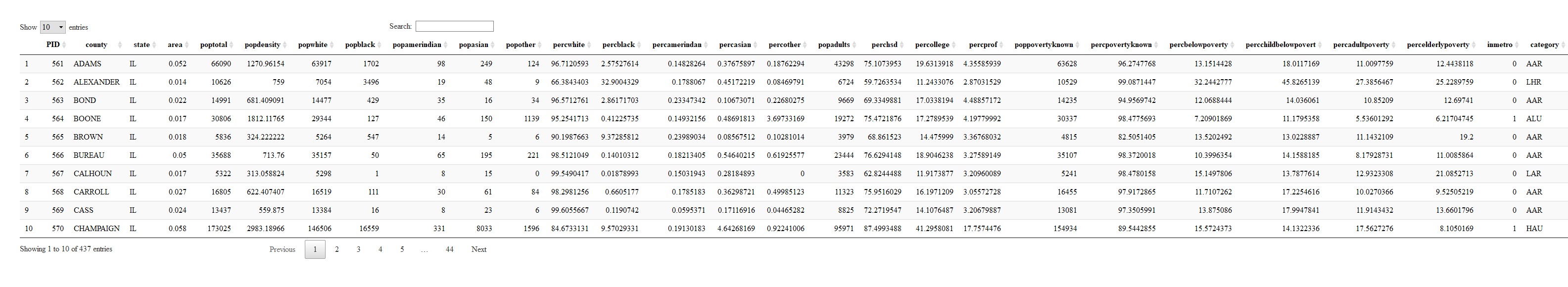
First ggplot

ggplot(data = midwest) +
  geom_point(mapping = aes(x = popdensity, y = percollege))

plot of chunk plot1

Equivalent Code

ggplot(midwest) +
  geom_point(aes(x = popdensity, y = percollege))

plot of chunk plot1_reduced

Your Turn

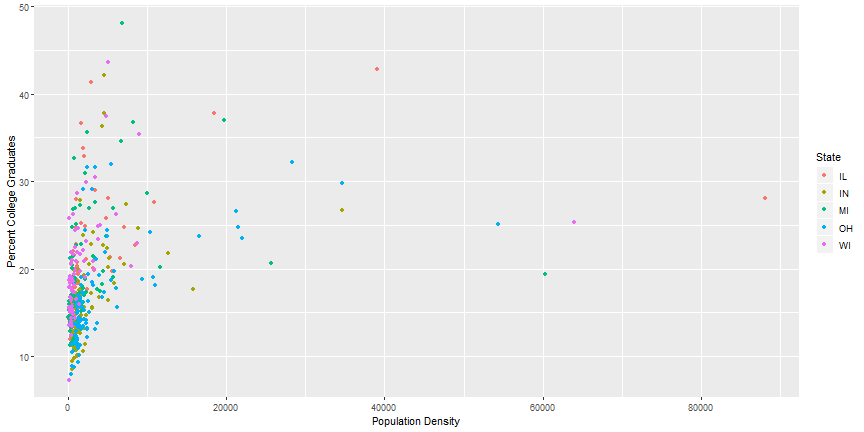
Try plotting popdensity by state.
Try plotting county by state.
- Does this plot work?
Bonus: Try just using the ggplot(data = midwest) from above.
- What do you get?
- Does this make sense?

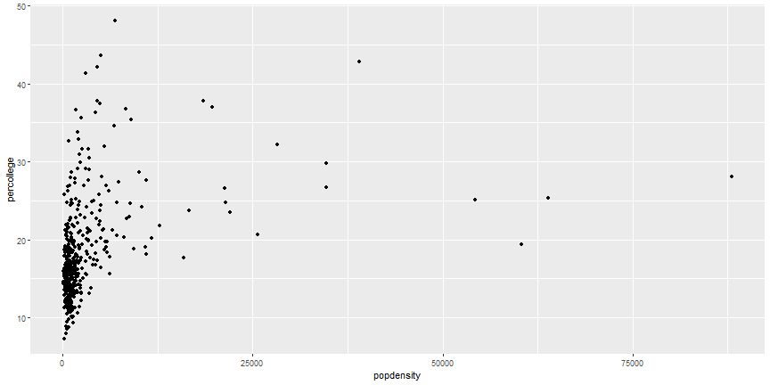
Add Aesthetics

ggplot(midwest) +
  geom_point(aes(x = popdensity, y = percollege, color = state))

plot of chunk aesthetic

Global Aesthetics

ggplot(midwest) +
  geom_point(aes(x = popdensity, y = percollege), color = 'pink')

plot of chunk global_aes

Your Turn

Instead of using colors, make the shape of the points different for each state.
Instead of color, use alpha instead.
- What does this do to the plot?
Try the following command: colors().
- Try a few colors to find your favorite.
What happens if you use the following code:

ggplot(midwest) + 
  geom_point(aes(x = popdensity, y = percollege, color = 'green'))

Additional Geoms

ggplot(midwest) +
  geom_smooth(aes(x = popdensity, y = percollege))

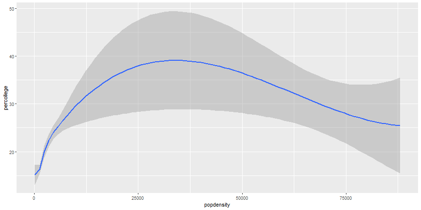
plot of chunk smooth

Add more Aesthetics

ggplot(midwest) +
  geom_smooth(aes(x = popdensity, y = percollege, linetype = state), 
              se = FALSE)

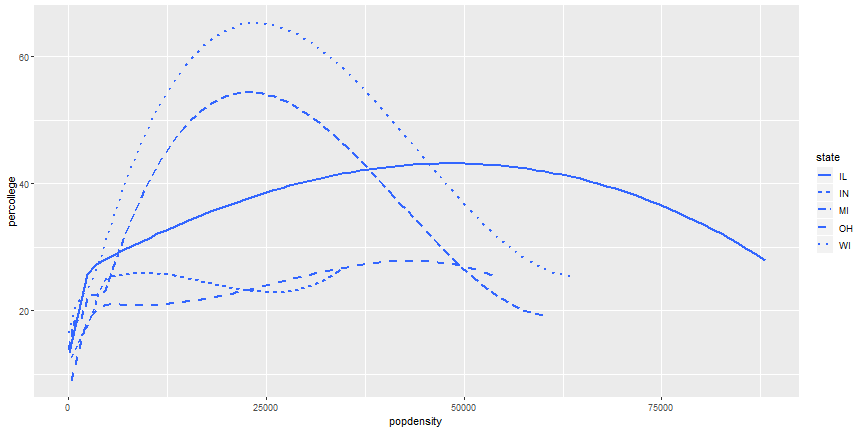
plot of chunk smooth_states

Your Turn

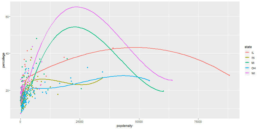
It is possible to combine geoms, which we will do next, but try it first. Try to recreate this plot.

Layered ggplot

ggplot(midwest) +
  geom_point(aes(x = popdensity, y = percollege, color = state)) +
  geom_smooth(aes(x = popdensity, y = percollege, color = state), 
              se = FALSE)

plot of chunk combine_geoms

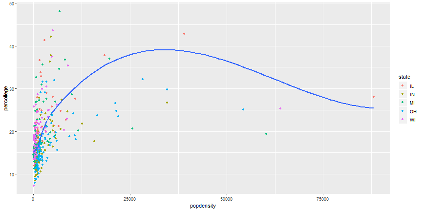
Remove duplicate aesthetics

ggplot(midwest, 
       aes(x = popdensity, y = percollege, color = state)) +
  geom_point() +
  geom_smooth(se = FALSE)

plot of chunk two_geoms

Your Turn

Can you recreate the following figure?

Brief plot customization

ggplot(midwest, 
       aes(x = popdensity, y = percollege, color = state)) +
  geom_point() + 
  scale_x_continuous("Population Density", 
                     breaks = seq(0, 80000, 20000)) + 
  scale_y_continuous("Percent College Graduates") + 
  scale_color_discrete("State")

Brief plot customization Output

plot of chunk breaks_x2

Additional ggplot2 resources

ggplot2 website: http://docs.ggplot2.org/current/index.html
ggplot2 book: http://www.springer.com/us/book/9780387981413
R graphics cookbook: http://www.cookbook-r.com/Graphs/

R works as a calculator

1 + 2 - 3

## [1] 0

5 * 7

## [1] 35

2/1

## [1] 2

R Calculator 2

sqrt(4)

## [1] 2

2^2

## [1] 4

Can save objects to use later

x <- 1 + 3
x

## [1] 4

x * 3

## [1] 12

R is case sensitive

case_sensitive <- 10
Case_sensitive

## Error in eval(expr, envir, enclos): object 'Case_sensitive' not found

R Functions

set.seed(1)
rnorm(n = 5, mean = 0, sd = 1)

## [1] -0.6264538  0.1836433 -0.8356286  1.5952808  0.3295078

set.seed(1)
rnorm(5, 0, 1)

## [1] -0.6264538  0.1836433 -0.8356286  1.5952808  0.3295078

set.seed(1)
rnorm(sd = 1, n = 5, mean = 0)

## [1] -0.6264538  0.1836433 -0.8356286  1.5952808  0.3295078

Working through Errors

Use ?function_name to explore the details of the function. The examples at the bottom of every R help page can be especially helpful.
- https://www.rdocumentation.org/ provided by DataCamp is a great alternative as well.
If this does not help, copy and paste the error and search on the internet.

Using `dplyr` for data manipulation

The dplyr package uses verbs for common data manipulation tasks. These include:

filter()
count()
arrange()
select()
mutate()
summarise()

Data

https://fivethirtyeight.com/features/both-republicans-and-democrats-have-an-age-problem/

install.packages('fivethirtyeight')
library(fivethirtyeight)

plot of chunk congress

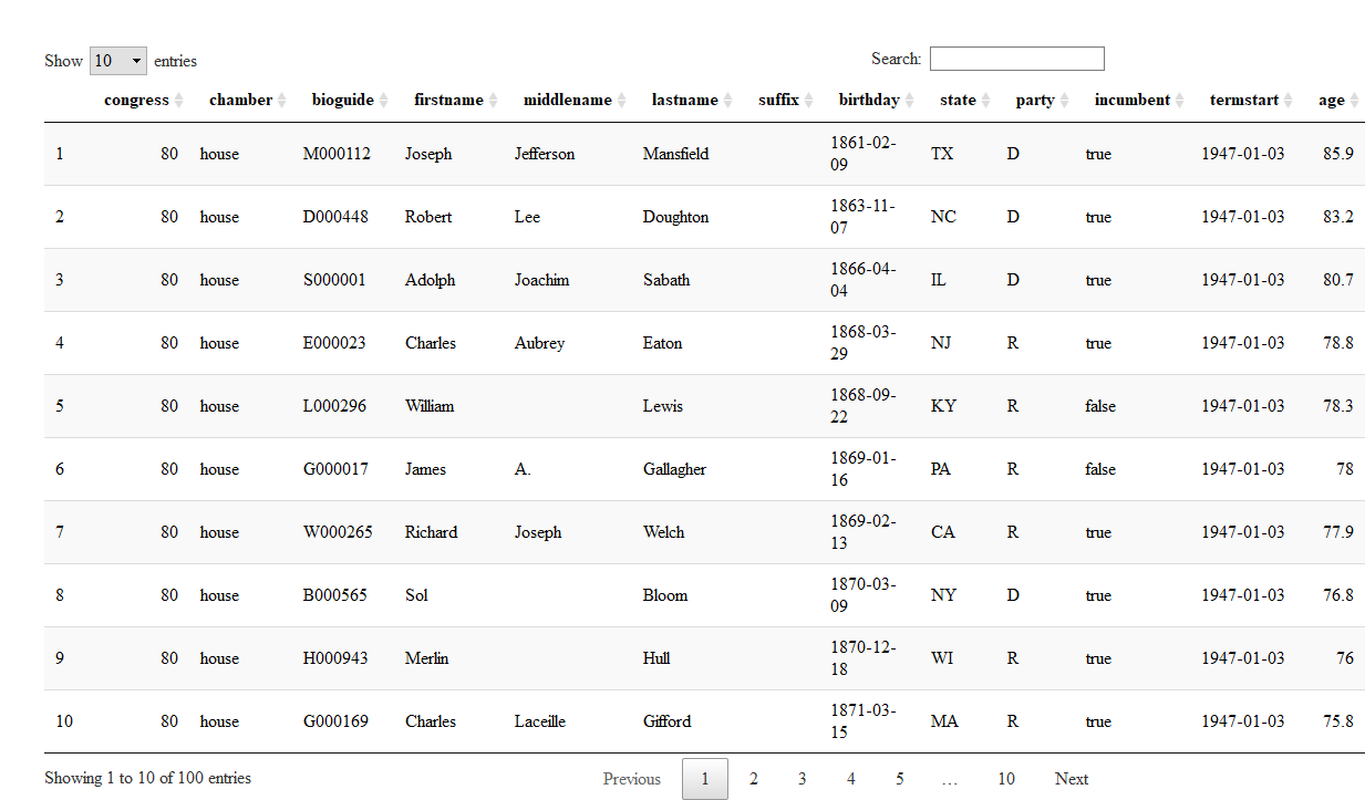
Using `filter`

filter(congress_age, congress == 80)

## # A tibble: 555 x 13
##    congress chamber bioguide firstname middlename  lastname suffix
##       <int>   <chr>    <chr>     <chr>      <chr>     <chr>  <chr>
##  1       80   house  M000112    Joseph  Jefferson Mansfield   <NA>
##  2       80   house  D000448    Robert        Lee  Doughton   <NA>
##  3       80   house  S000001    Adolph    Joachim    Sabath   <NA>
##  4       80   house  E000023   Charles     Aubrey     Eaton   <NA>
##  5       80   house  L000296   William       <NA>     Lewis   <NA>
##  6       80   house  G000017     James         A. Gallagher   <NA>
##  7       80   house  W000265   Richard     Joseph     Welch   <NA>
##  8       80   house  B000565       Sol       <NA>     Bloom   <NA>
##  9       80   house  H000943    Merlin       <NA>      Hull   <NA>
## 10       80   house  G000169   Charles   Laceille   Gifford   <NA>
## # ... with 545 more rows, and 6 more variables: birthday <date>,
## #   state <chr>, party <chr>, incumbent <lgl>, termstart <date>, age <dbl>

Save filtered results to object

congress_80 <- filter(congress_age, congress == 80)

Other operators for numbers

>
<
>=
<=

Your Turn

Select all rows where the congress member was older than 80 at the start of the term.
Use the is.na function to identify congress members that have missing middlenames.

Filter character variables

senate <- filter(congress_age, chamber == 'senate')

Combine Operations - AND

filter(congress_age, congress == 80, chamber == 'senate')

## # A tibble: 102 x 13
##    congress chamber bioguide firstname middlename lastname suffix
##       <int>   <chr>    <chr>     <chr>      <chr>    <chr>  <chr>
##  1       80  senate  C000133    Arthur       <NA>   Capper   <NA>
##  2       80  senate  G000418  Theodore    Francis    Green   <NA>
##  3       80  senate  M000499   Kenneth    Douglas McKellar   <NA>
##  4       80  senate  R000112     Clyde     Martin     Reed   <NA>
##  5       80  senate  M000895    Edward       Hall    Moore   <NA>
##  6       80  senate  O000146      John     Holmes  Overton   <NA>
##  7       80  senate  M001108     James     Edward   Murray   <NA>
##  8       80  senate  M000308   Patrick    Anthony McCarran   <NA>
##  9       80  senate  T000165     Elmer       <NA>   Thomas   <NA>
## 10       80  senate  W000021    Robert  Ferdinand   Wagner   <NA>
## # ... with 92 more rows, and 6 more variables: birthday <date>,
## #   state <chr>, party <chr>, incumbent <lgl>, termstart <date>, age <dbl>

Equivalent AND Statement

filter(congress_age, congress == 80 & chamber == 'senate')

## # A tibble: 102 x 13
##    congress chamber bioguide firstname middlename lastname suffix
##       <int>   <chr>    <chr>     <chr>      <chr>    <chr>  <chr>
##  1       80  senate  C000133    Arthur       <NA>   Capper   <NA>
##  2       80  senate  G000418  Theodore    Francis    Green   <NA>
##  3       80  senate  M000499   Kenneth    Douglas McKellar   <NA>
##  4       80  senate  R000112     Clyde     Martin     Reed   <NA>
##  5       80  senate  M000895    Edward       Hall    Moore   <NA>
##  6       80  senate  O000146      John     Holmes  Overton   <NA>
##  7       80  senate  M001108     James     Edward   Murray   <NA>
##  8       80  senate  M000308   Patrick    Anthony McCarran   <NA>
##  9       80  senate  T000165     Elmer       <NA>   Thomas   <NA>
## 10       80  senate  W000021    Robert  Ferdinand   Wagner   <NA>
## # ... with 92 more rows, and 6 more variables: birthday <date>,
## #   state <chr>, party <chr>, incumbent <lgl>, termstart <date>, age <dbl>

Filter - OR

filter(congress_age, congress == 80 | congress == 81)

## # A tibble: 1,112 x 13
##    congress chamber bioguide firstname middlename  lastname suffix
##       <int>   <chr>    <chr>     <chr>      <chr>     <chr>  <chr>
##  1       80   house  M000112    Joseph  Jefferson Mansfield   <NA>
##  2       80   house  D000448    Robert        Lee  Doughton   <NA>
##  3       80   house  S000001    Adolph    Joachim    Sabath   <NA>
##  4       80   house  E000023   Charles     Aubrey     Eaton   <NA>
##  5       80   house  L000296   William       <NA>     Lewis   <NA>
##  6       80   house  G000017     James         A. Gallagher   <NA>
##  7       80   house  W000265   Richard     Joseph     Welch   <NA>
##  8       80   house  B000565       Sol       <NA>     Bloom   <NA>
##  9       80   house  H000943    Merlin       <NA>      Hull   <NA>
## 10       80   house  G000169   Charles   Laceille   Gifford   <NA>
## # ... with 1,102 more rows, and 6 more variables: birthday <date>,
## #   state <chr>, party <chr>, incumbent <lgl>, termstart <date>, age <dbl>

`%in%`

filter(congress_age, congress %in% c(80, 81))

## # A tibble: 1,112 x 13
##    congress chamber bioguide firstname middlename  lastname suffix
##       <int>   <chr>    <chr>     <chr>      <chr>     <chr>  <chr>
##  1       80   house  M000112    Joseph  Jefferson Mansfield   <NA>
##  2       80   house  D000448    Robert        Lee  Doughton   <NA>
##  3       80   house  S000001    Adolph    Joachim    Sabath   <NA>
##  4       80   house  E000023   Charles     Aubrey     Eaton   <NA>
##  5       80   house  L000296   William       <NA>     Lewis   <NA>
##  6       80   house  G000017     James         A. Gallagher   <NA>
##  7       80   house  W000265   Richard     Joseph     Welch   <NA>
##  8       80   house  B000565       Sol       <NA>     Bloom   <NA>
##  9       80   house  H000943    Merlin       <NA>      Hull   <NA>
## 10       80   house  G000169   Charles   Laceille   Gifford   <NA>
## # ... with 1,102 more rows, and 6 more variables: birthday <date>,
## #   state <chr>, party <chr>, incumbent <lgl>, termstart <date>, age <dbl>

Not Operator

filter(congress_age, congress != 80)

## # A tibble: 18,080 x 13
##    congress chamber bioguide firstname middlename lastname suffix
##       <int>   <chr>    <chr>     <chr>      <chr>    <chr>  <chr>
##  1       81   house  D000448    Robert        Lee Doughton   <NA>
##  2       81   house  S000001    Adolph    Joachim   Sabath   <NA>
##  3       81   house  E000023   Charles     Aubrey    Eaton   <NA>
##  4       81   house  W000265   Richard     Joseph    Welch   <NA>
##  5       81   house  B000565       Sol       <NA>    Bloom   <NA>
##  6       81   house  H000943    Merlin       <NA>     Hull   <NA>
##  7       81   house  B000545  Schuyler       Otis    Bland   <NA>
##  8       81   house  K000138      John      Hosea     Kerr   <NA>
##  9       81   house  C000932    Robert       <NA>  Crosser   <NA>
## 10       81   house  K000039      John       <NA>      Kee   <NA>
## # ... with 18,070 more rows, and 6 more variables: birthday <date>,
## #   state <chr>, party <chr>, incumbent <lgl>, termstart <date>, age <dbl>

Not Operator 2

filter(congress_age, congress == 80 & !chamber == 'senate')

## # A tibble: 453 x 13
##    congress chamber bioguide firstname middlename  lastname suffix
##       <int>   <chr>    <chr>     <chr>      <chr>     <chr>  <chr>
##  1       80   house  M000112    Joseph  Jefferson Mansfield   <NA>
##  2       80   house  D000448    Robert        Lee  Doughton   <NA>
##  3       80   house  S000001    Adolph    Joachim    Sabath   <NA>
##  4       80   house  E000023   Charles     Aubrey     Eaton   <NA>
##  5       80   house  L000296   William       <NA>     Lewis   <NA>
##  6       80   house  G000017     James         A. Gallagher   <NA>
##  7       80   house  W000265   Richard     Joseph     Welch   <NA>
##  8       80   house  B000565       Sol       <NA>     Bloom   <NA>
##  9       80   house  H000943    Merlin       <NA>      Hull   <NA>
## 10       80   house  G000169   Charles   Laceille   Gifford   <NA>
## # ... with 443 more rows, and 6 more variables: birthday <date>,
## #   state <chr>, party <chr>, incumbent <lgl>, termstart <date>, age <dbl>

Working with logicals

filter(congress_age, incumbent)

## # A tibble: 15,698 x 13
##    congress chamber bioguide firstname middlename  lastname suffix
##       <int>   <chr>    <chr>     <chr>      <chr>     <chr>  <chr>
##  1       80   house  M000112    Joseph  Jefferson Mansfield   <NA>
##  2       80   house  D000448    Robert        Lee  Doughton   <NA>
##  3       80   house  S000001    Adolph    Joachim    Sabath   <NA>
##  4       80   house  E000023   Charles     Aubrey     Eaton   <NA>
##  5       80   house  W000265   Richard     Joseph     Welch   <NA>
##  6       80   house  B000565       Sol       <NA>     Bloom   <NA>
##  7       80   house  H000943    Merlin       <NA>      Hull   <NA>
##  8       80   house  G000169   Charles   Laceille   Gifford   <NA>
##  9       80   house  B000545  Schuyler       Otis     Bland   <NA>
## 10       80   house  R000358      John   Marshall   Robsion   <NA>
## # ... with 15,688 more rows, and 6 more variables: birthday <date>,
## #   state <chr>, party <chr>, incumbent <lgl>, termstart <date>, age <dbl>

Your Turn

Select the Senators from Iowa.
Select the Senators from Iowa that are not inbumbents.

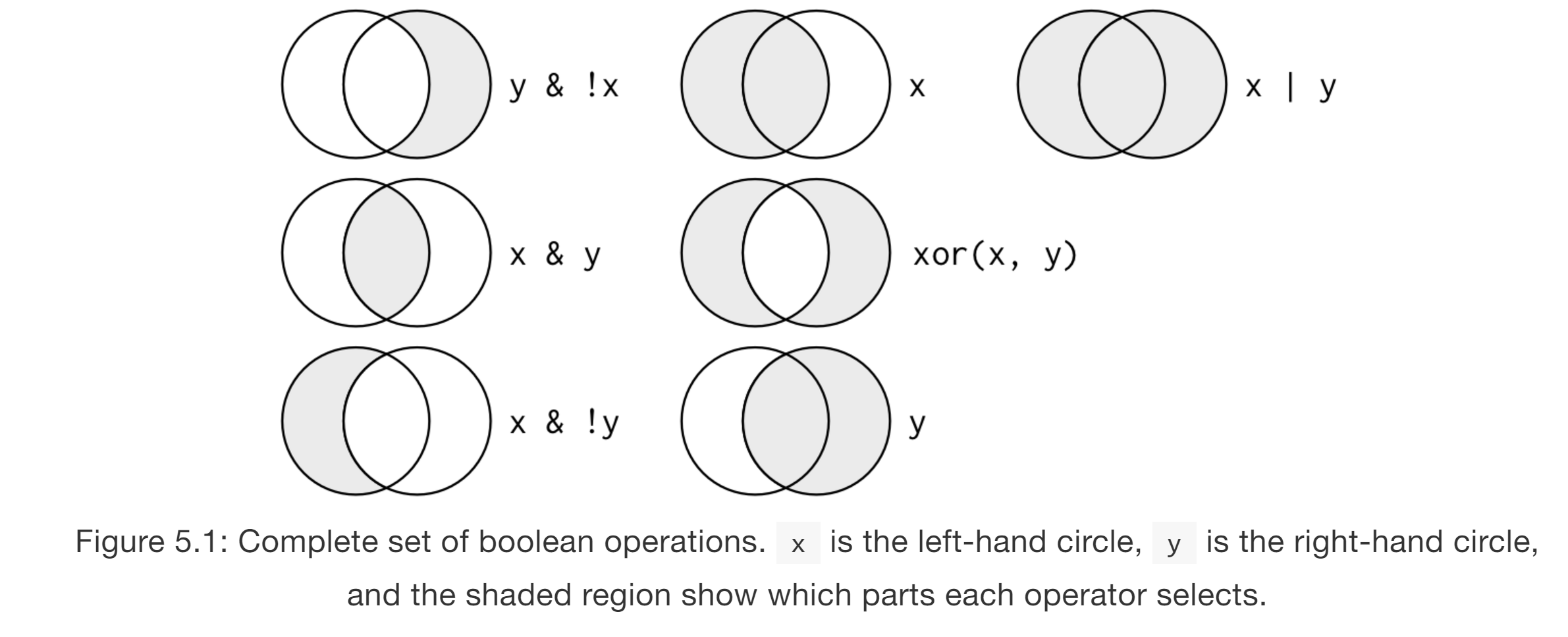
All boolean options

Using `count`

count(congress_age, party)

## # A tibble: 6 x 2
##   party     n
##   <chr> <int>
## 1    AL     3
## 2     D 10290
## 3     I    63
## 4    ID     4
## 5     L     1
## 6     R  8274

count(congress_age, incumbent)

## # A tibble: 2 x 2
##   incumbent     n
##       <lgl> <int>
## 1     FALSE  2937
## 2      TRUE 15698

Using `arrange`

arrange(congress_age, state)

## # A tibble: 18,635 x 13
##    congress chamber bioguide firstname middlename lastname suffix
##       <int>   <chr>    <chr>     <chr>      <chr>    <chr>  <chr>
##  1       80   house  B000201    Edward      Lewis Bartlett   <NA>
##  2       81   house  B000201    Edward      Lewis Bartlett   <NA>
##  3       82   house  B000201    Edward      Lewis Bartlett   <NA>
##  4       83   house  B000201    Edward      Lewis Bartlett   <NA>
##  5       84   house  B000201    Edward      Lewis Bartlett   <NA>
##  6       85   house  B000201    Edward      Lewis Bartlett   <NA>
##  7       86   house  R000282     Ralph     Julian   Rivers   <NA>
##  8       86  senate  G000508    Ernest       <NA> Gruening   <NA>
##  9       86  senate  B000201    Edward      Lewis Bartlett   <NA>
## 10       87   house  R000282     Ralph     Julian   Rivers   <NA>
## # ... with 18,625 more rows, and 6 more variables: birthday <date>,
## #   state <chr>, party <chr>, incumbent <lgl>, termstart <date>, age <dbl>

Add more variables

arrange(congress_age, state, party)

## # A tibble: 18,635 x 13
##    congress chamber bioguide firstname middlename lastname suffix
##       <int>   <chr>    <chr>     <chr>      <chr>    <chr>  <chr>
##  1       80   house  B000201    Edward      Lewis Bartlett   <NA>
##  2       81   house  B000201    Edward      Lewis Bartlett   <NA>
##  3       82   house  B000201    Edward      Lewis Bartlett   <NA>
##  4       83   house  B000201    Edward      Lewis Bartlett   <NA>
##  5       84   house  B000201    Edward      Lewis Bartlett   <NA>
##  6       85   house  B000201    Edward      Lewis Bartlett   <NA>
##  7       86   house  R000282     Ralph     Julian   Rivers   <NA>
##  8       86  senate  G000508    Ernest       <NA> Gruening   <NA>
##  9       86  senate  B000201    Edward      Lewis Bartlett   <NA>
## 10       87   house  R000282     Ralph     Julian   Rivers   <NA>
## # ... with 18,625 more rows, and 6 more variables: birthday <date>,
## #   state <chr>, party <chr>, incumbent <lgl>, termstart <date>, age <dbl>

Descending Order

arrange(congress_age, desc(congress))

## # A tibble: 18,635 x 13
##    congress chamber bioguide firstname middlename  lastname suffix
##       <int>   <chr>    <chr>     <chr>      <chr>     <chr>  <chr>
##  1      113   house  H000067     Ralph         M.      Hall   <NA>
##  2      113   house  D000355      John         D.   Dingell   <NA>
##  3      113   house  C000714      John       <NA>   Conyers    Jr.
##  4      113   house  S000480    Louise   McIntosh Slaughter   <NA>
##  5      113   house  R000053   Charles         B.    Rangel   <NA>
##  6      113   house  J000174       Sam     Robert   Johnson   <NA>
##  7      113   house  Y000031        C.    W. Bill     Young   <NA>
##  8      113   house  C000556    Howard       <NA>     Coble   <NA>
##  9      113   house  L000263    Sander         M.     Levin   <NA>
## 10      113   house  Y000033       Don         E.     Young   <NA>
## # ... with 18,625 more rows, and 6 more variables: birthday <date>,
## #   state <chr>, party <chr>, incumbent <lgl>, termstart <date>, age <dbl>

Your Turn

Count the number of congress members from each party that are older than 80 at term start.
Arrange the result from above by the variable n.

Using `select`

select(congress_age, congress, chamber, party, age)

## # A tibble: 18,635 x 4
##    congress chamber party   age
##       <int>   <chr> <chr> <dbl>
##  1       80   house     D  85.9
##  2       80   house     D  83.2
##  3       80   house     D  80.7
##  4       80   house     R  78.8
##  5       80   house     R  78.3
##  6       80   house     R  78.0
##  7       80   house     R  77.9
##  8       80   house     D  76.8
##  9       80   house     R  76.0
## 10       80   house     R  75.8
## # ... with 18,625 more rows

Helper functions

starts_with()
ends_with()
contains()
matches()
num_range()
:
everything()

`starts_with` helper

select(congress_age, starts_with('s'))

## # A tibble: 18,635 x 2
##    suffix state
##     <chr> <chr>
##  1   <NA>    TX
##  2   <NA>    NC
##  3   <NA>    IL
##  4   <NA>    NJ
##  5   <NA>    KY
##  6   <NA>    PA
##  7   <NA>    CA
##  8   <NA>    NY
##  9   <NA>    WI
## 10   <NA>    MA
## # ... with 18,625 more rows

Contains helper

select(congress_age, contains('name'))

## # A tibble: 18,635 x 3
##    firstname middlename  lastname
##        <chr>      <chr>     <chr>
##  1    Joseph  Jefferson Mansfield
##  2    Robert        Lee  Doughton
##  3    Adolph    Joachim    Sabath
##  4   Charles     Aubrey     Eaton
##  5   William       <NA>     Lewis
##  6     James         A. Gallagher
##  7   Richard     Joseph     Welch
##  8       Sol       <NA>     Bloom
##  9    Merlin       <NA>      Hull
## 10   Charles   Laceille   Gifford
## # ... with 18,625 more rows

Colon

select(congress_age, congress:birthday)

## # A tibble: 18,635 x 8
##    congress chamber bioguide firstname middlename  lastname suffix
##       <int>   <chr>    <chr>     <chr>      <chr>     <chr>  <chr>
##  1       80   house  M000112    Joseph  Jefferson Mansfield   <NA>
##  2       80   house  D000448    Robert        Lee  Doughton   <NA>
##  3       80   house  S000001    Adolph    Joachim    Sabath   <NA>
##  4       80   house  E000023   Charles     Aubrey     Eaton   <NA>
##  5       80   house  L000296   William       <NA>     Lewis   <NA>
##  6       80   house  G000017     James         A. Gallagher   <NA>
##  7       80   house  W000265   Richard     Joseph     Welch   <NA>
##  8       80   house  B000565       Sol       <NA>     Bloom   <NA>
##  9       80   house  H000943    Merlin       <NA>      Hull   <NA>
## 10       80   house  G000169   Charles   Laceille   Gifford   <NA>
## # ... with 18,625 more rows, and 1 more variables: birthday <date>

Drop variables

select(congress_age, -firstname, -state, -party, -incumbent, -chamber)

## # A tibble: 18,635 x 8
##    congress bioguide middlename  lastname suffix   birthday  termstart
##       <int>    <chr>      <chr>     <chr>  <chr>     <date>     <date>
##  1       80  M000112  Jefferson Mansfield   <NA> 1861-02-09 1947-01-03
##  2       80  D000448        Lee  Doughton   <NA> 1863-11-07 1947-01-03
##  3       80  S000001    Joachim    Sabath   <NA> 1866-04-04 1947-01-03
##  4       80  E000023     Aubrey     Eaton   <NA> 1868-03-29 1947-01-03
##  5       80  L000296       <NA>     Lewis   <NA> 1868-09-22 1947-01-03
##  6       80  G000017         A. Gallagher   <NA> 1869-01-16 1947-01-03
##  7       80  W000265     Joseph     Welch   <NA> 1869-02-13 1947-01-03
##  8       80  B000565       <NA>     Bloom   <NA> 1870-03-09 1947-01-03
##  9       80  H000943       <NA>      Hull   <NA> 1870-12-18 1947-01-03
## 10       80  G000169   Laceille   Gifford   <NA> 1871-03-15 1947-01-03
## # ... with 18,625 more rows, and 1 more variables: age <dbl>

Reorder with `everything`

select(congress_age, congress, chamber, incumbent, age, everything())

## # A tibble: 18,635 x 13
##    congress chamber incumbent   age bioguide firstname middlename
##       <int>   <chr>     <lgl> <dbl>    <chr>     <chr>      <chr>
##  1       80   house      TRUE  85.9  M000112    Joseph  Jefferson
##  2       80   house      TRUE  83.2  D000448    Robert        Lee
##  3       80   house      TRUE  80.7  S000001    Adolph    Joachim
##  4       80   house      TRUE  78.8  E000023   Charles     Aubrey
##  5       80   house     FALSE  78.3  L000296   William       <NA>
##  6       80   house     FALSE  78.0  G000017     James         A.
##  7       80   house      TRUE  77.9  W000265   Richard     Joseph
##  8       80   house      TRUE  76.8  B000565       Sol       <NA>
##  9       80   house      TRUE  76.0  H000943    Merlin       <NA>
## 10       80   house      TRUE  75.8  G000169   Charles   Laceille
## # ... with 18,625 more rows, and 6 more variables: lastname <chr>,
## #   suffix <chr>, birthday <date>, state <chr>, party <chr>,
## #   termstart <date>

`rename` function

rename(congress_age, first_name = firstname, last_name = lastname)

## # A tibble: 18,635 x 13
##    congress chamber bioguide first_name middlename last_name suffix
##       <int>   <chr>    <chr>      <chr>      <chr>     <chr>  <chr>
##  1       80   house  M000112     Joseph  Jefferson Mansfield   <NA>
##  2       80   house  D000448     Robert        Lee  Doughton   <NA>
##  3       80   house  S000001     Adolph    Joachim    Sabath   <NA>
##  4       80   house  E000023    Charles     Aubrey     Eaton   <NA>
##  5       80   house  L000296    William       <NA>     Lewis   <NA>
##  6       80   house  G000017      James         A. Gallagher   <NA>
##  7       80   house  W000265    Richard     Joseph     Welch   <NA>
##  8       80   house  B000565        Sol       <NA>     Bloom   <NA>
##  9       80   house  H000943     Merlin       <NA>      Hull   <NA>
## 10       80   house  G000169    Charles   Laceille   Gifford   <NA>
## # ... with 18,625 more rows, and 6 more variables: birthday <date>,
## #   state <chr>, party <chr>, incumbent <lgl>, termstart <date>, age <dbl>

Your Turn

Using the dplyr helper functions, select all the variables that start with the letter ‘c’.
Rename the first three variables in the congress data to ‘x1’, ‘x2’, ‘x3’.
After renaming the first three variables, use this new data (ensure you saved the previous step to an object) to select these three variables with the num_range function.

Using `mutate`

congress_red <- select(congress_age, congress, chamber, state, party)

mutate(congress_red, 
       democrat = ifelse(party == 'D', 1, 0),
       num_democrat = sum(democrat)
       )

## # A tibble: 18,635 x 6
##    congress chamber state party democrat num_democrat
##       <int>   <chr> <chr> <chr>    <dbl>        <dbl>
##  1       80   house    TX     D        1        10290
##  2       80   house    NC     D        1        10290
##  3       80   house    IL     D        1        10290
##  4       80   house    NJ     R        0        10290
##  5       80   house    KY     R        0        10290
##  6       80   house    PA     R        0        10290
##  7       80   house    CA     R        0        10290
##  8       80   house    NY     D        1        10290
##  9       80   house    WI     R        0        10290
## 10       80   house    MA     R        0        10290
## # ... with 18,625 more rows

Your Turn

Using the diamonds data, use ?diamonds for more information on the data, use the mutate function to calculate the price per carat. Hint, this operation would involve standardizing the price variable so that all are comparable at 1 carat.
Using mutate, calculate the rank of the original price variable and the new price variable calculated above using the min_rank function. Are there differences in the ranking of the prices?

Using `summarise`

congress_2 <- mutate(congress_age, 
       democrat = ifelse(party == 'D', 1, 0)
       )

summarise(congress_2, 
          num_democrat = sum(democrat)
          )

## # A tibble: 1 x 1
##   num_democrat
##          <dbl>
## 1        10290

`group_by`

congress_grp <- group_by(congress_2, congress)

summarise(congress_grp, 
          num_democrat = sum(democrat),
          total = n(),
          prop_democrat = num_democrat / total
)

## # A tibble: 34 x 4
##    congress num_democrat total prop_democrat
##       <int>        <dbl> <int>         <dbl>
##  1       80          247   555     0.4450450
##  2       81          330   557     0.5924596
##  3       82          292   555     0.5261261
##  4       83          274   557     0.4919210
##  5       84          288   544     0.5294118
##  6       85          295   547     0.5393053
##  7       86          356   554     0.6425993
##  8       87          339   559     0.6064401
##  9       88          332   552     0.6014493
## 10       89          371   548     0.6770073
## # ... with 24 more rows

Explore trend

num_dem <- summarise(congress_grp, 
                     num_democrat = sum(democrat),
                     total = n(),
                     prop_democrat = num_democrat / total
)
ggplot(num_dem, aes(x = congress, y = prop_democrat)) + 
  geom_line()

Explore trend output

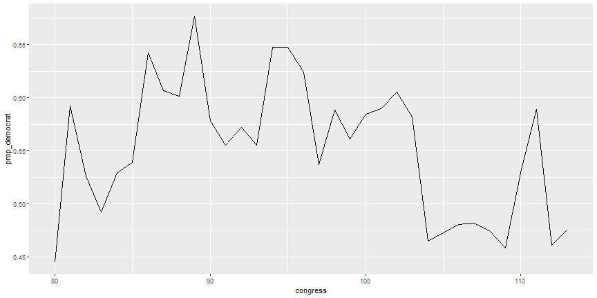
plot of chunk trend2

Your Turn

Suppose we wanted to calculate the number and proportion of republicans instead of democrats, assuming these are the only two parties, edit the summarise command above to calculate these values.
Suppose instead of using sum(democrat) above, we used mean(democrat), what does this value return? Why does it return this value?

`group_by` with `mutate`

congress_red <- select(congress_age, congress, chamber, state, party)
congress_grp <- group_by(congress_red, congress)

mutate(congress_grp, 
       democrat = ifelse(party == 'D', 1, 0),
       num_democrat = sum(democrat),
       total = n(),
       prop_democrat = num_democrat / total
)

`group_by` with `mutate` output

## # A tibble: 18,635 x 8
## # Groups:   congress [34]
##    congress chamber state party democrat num_democrat total prop_democrat
##       <int>   <chr> <chr> <chr>    <dbl>        <dbl> <int>         <dbl>
##  1       80   house    TX     D        1          247   555      0.445045
##  2       80   house    NC     D        1          247   555      0.445045
##  3       80   house    IL     D        1          247   555      0.445045
##  4       80   house    NJ     R        0          247   555      0.445045
##  5       80   house    KY     R        0          247   555      0.445045
##  6       80   house    PA     R        0          247   555      0.445045
##  7       80   house    CA     R        0          247   555      0.445045
##  8       80   house    NY     D        1          247   555      0.445045
##  9       80   house    WI     R        0          247   555      0.445045
## 10       80   house    MA     R        0          247   555      0.445045
## # ... with 18,625 more rows

Chaining operations

summarise(
  group_by(
    mutate(
      filter(
        congress_age, congress >= 100
      ), 
      democrat = ifelse(party == 'D', 1, 0)
    ),
    congress, chamber
  ),
  num_democrat = sum(democrat),
  total = n(),
  prop_democrat = num_democrat / total
)

The pipe `%>%` is the answer

congress_age %>%
  filter(congress >= 100) %>%
  mutate(democrat = ifelse(party == 'D', 1, 0)) %>%
  group_by(congress, chamber) %>%
  summarise(
    num_democrat = sum(democrat),
    total = n(),
    prop_democrat = num_democrat / total
  )

The two are identical

pipe_congress <- congress_age %>%
  filter(congress >= 100) %>%
  mutate(democrat = ifelse(party == 'D', 1, 0)) %>%
  group_by(congress, chamber) %>%
  summarise(
    num_democrat = sum(democrat),
    total = n(),
    prop_democrat = num_democrat / total
  )

nested_congress <- summarise(
  group_by(
    mutate(
      filter(
        congress_age, congress >= 100
      ), 
      democrat = ifelse(party == 'D', 1, 0)
    ),
    congress, chamber
  ),
  num_democrat = sum(democrat),
  total = n(),
  prop_democrat = num_democrat / total
)

identical(pipe_congress, nested_congress)

## [1] TRUE

Your Turn

Look at the following nested code and determine what is being done. Then translate this code to use the pipe operator.

summarise(
  group_by(
    mutate(
      filter(
        diamonds, 
        color %in% c('D', 'E', 'F') & cut %in% c('Fair', 'Good', 'Very Good')
      ),
      f_color = ifelse(color == 'F', 1, 0),
      vg_cut = ifelse(cut == 'Very Good', 1, 0)
    ),
    clarity
  ),
  avg = mean(carat),
  sd = sd(carat),
  avg_p = mean(price),
  num = n(),
  summary_f_color = mean(f_color),
  summary_vg_cut = mean(vg_cut)
)

Other Useful dplyr functions

There are a set of functions that can greatly simplify data operations. These functions end with:

*_if
*_each
*_all
*_at

Simple example

rename_if(congress_age, is.character, toupper)

## # A tibble: 18,635 x 13
##    congress CHAMBER BIOGUIDE FIRSTNAME MIDDLENAME  LASTNAME SUFFIX
##       <int>   <chr>    <chr>     <chr>      <chr>     <chr>  <chr>
##  1       80   house  M000112    Joseph  Jefferson Mansfield   <NA>
##  2       80   house  D000448    Robert        Lee  Doughton   <NA>
##  3       80   house  S000001    Adolph    Joachim    Sabath   <NA>
##  4       80   house  E000023   Charles     Aubrey     Eaton   <NA>
##  5       80   house  L000296   William       <NA>     Lewis   <NA>
##  6       80   house  G000017     James         A. Gallagher   <NA>
##  7       80   house  W000265   Richard     Joseph     Welch   <NA>
##  8       80   house  B000565       Sol       <NA>     Bloom   <NA>
##  9       80   house  H000943    Merlin       <NA>      Hull   <NA>
## 10       80   house  G000169   Charles   Laceille   Gifford   <NA>
## # ... with 18,625 more rows, and 6 more variables: birthday <date>,
## #   STATE <chr>, PARTY <chr>, incumbent <lgl>, termstart <date>, age <dbl>

More realistic example

starwars %>%
  group_by(species, gender) %>%
  summarise_if(is.numeric, mean, na.rm = TRUE)

## # A tibble: 43 x 5
## # Groups:   species [?]
##      species gender height      mass birth_year
##        <chr>  <chr>  <dbl>     <dbl>      <dbl>
##  1    Aleena   male     79  15.00000        NaN
##  2  Besalisk   male    198 102.00000        NaN
##  3    Cerean   male    198  82.00000       92.0
##  4  Chagrian   male    196       NaN        NaN
##  5  Clawdite female    168  55.00000        NaN
##  6     Droid   none    200 140.00000       15.0
##  7     Droid   <NA>    120  46.33333       72.5
##  8       Dug   male    112  40.00000        NaN
##  9      Ewok   male     88  20.00000        8.0
## 10 Geonosian   male    183  80.00000        NaN
## # ... with 33 more rows

Can call more than one function

starwars %>%
  group_by(species, gender) %>%
  summarise_if(is.numeric, funs(mean, median), na.rm = TRUE) %>%
  add_tally()

## # A tibble: 43 x 9
## # Groups:   species [38]
##      species gender height_mean mass_mean birth_year_mean height_median
##        <chr>  <chr>       <dbl>     <dbl>           <dbl>         <dbl>
##  1    Aleena   male          79  15.00000             NaN            79
##  2  Besalisk   male         198 102.00000             NaN           198
##  3    Cerean   male         198  82.00000            92.0           198
##  4  Chagrian   male         196       NaN             NaN           196
##  5  Clawdite female         168  55.00000             NaN           168
##  6     Droid   none         200 140.00000            15.0           200
##  7     Droid   <NA>         120  46.33333            72.5            97
##  8       Dug   male         112  40.00000             NaN           112
##  9      Ewok   male          88  20.00000             8.0            88
## 10 Geonosian   male         183  80.00000             NaN           183
## # ... with 33 more rows, and 3 more variables: mass_median <dbl>,
## #   birth_year_median <dbl>, n <int>

Read in your own data

We will use data posted to GitHub: https://github.com/lebebr01/iowa_data_science/tree/master/data

Data Import

ufo <- read_csv("https://raw.githubusercontent.com/lebebr01/iowa_data_science/master/data/ufo.csv")

## Parsed with column specification:
## cols(
##   `Date / Time` = col_character(),
##   City = col_character(),
##   State = col_character(),
##   Shape = col_character(),
##   Duration = col_character(),
##   Summary = col_character(),
##   Posted = col_character()
## )

Show Data

ufo

## # A tibble: 8,031 x 7
##     `Date / Time`                     City State    Shape    Duration
##             <chr>                    <chr> <chr>    <chr>       <chr>
##  1 12/12/14 17:30              North Wales    PA Triangle   5 minutes
##  2 12/12/14 12:40             Cartersville    GA  Unknown 3.6 minutes
##  3 12/12/14 06:30 Isle of Man (UK/England)  <NA>    Light   2 seconds
##  4 12/12/14 01:00               Miamisburg    OH Changing        <NA>
##  5 12/12/14 00:00             Spotsylvania    VA  Unknown    1 minute
##  6 12/11/14 23:25                   Kenner    LA  Chevron   ~1 minute
##  7 12/11/14 23:15                   Eugene    OR     Disk   2 minutes
##  8 12/11/14 20:04                  Phoenix    AZ  Chevron   3 minutes
##  9 12/11/14 20:00                 Franklin    NC     Disk   5 minutes
## 10 12/11/14 18:30                 Longview    WA Cylinder  10 seconds
## # ... with 8,021 more rows, and 2 more variables: Summary <chr>,
## #   Posted <chr>

Manual column names

ufo_man <- read_csv("https://raw.githubusercontent.com/lebebr01/iowa_data_science/master/data/ufo.csv", 
         skip = 1, 
         col_names = c('Date/Time', 'City', 'State', 
                       'Shape', 'Duration', 'Summary',
                       'Posted'))

## Parsed with column specification:
## cols(
##   `Date/Time` = col_character(),
##   City = col_character(),
##   State = col_character(),
##   Shape = col_character(),
##   Duration = col_character(),
##   Summary = col_character(),
##   Posted = col_character()
## )

Manual column names output

ufo_man

## # A tibble: 8,031 x 7
##       `Date/Time`                     City State    Shape    Duration
##             <chr>                    <chr> <chr>    <chr>       <chr>
##  1 12/12/14 17:30              North Wales    PA Triangle   5 minutes
##  2 12/12/14 12:40             Cartersville    GA  Unknown 3.6 minutes
##  3 12/12/14 06:30 Isle of Man (UK/England)  <NA>    Light   2 seconds
##  4 12/12/14 01:00               Miamisburg    OH Changing        <NA>
##  5 12/12/14 00:00             Spotsylvania    VA  Unknown    1 minute
##  6 12/11/14 23:25                   Kenner    LA  Chevron   ~1 minute
##  7 12/11/14 23:15                   Eugene    OR     Disk   2 minutes
##  8 12/11/14 20:04                  Phoenix    AZ  Chevron   3 minutes
##  9 12/11/14 20:00                 Franklin    NC     Disk   5 minutes
## 10 12/11/14 18:30                 Longview    WA Cylinder  10 seconds
## # ... with 8,021 more rows, and 2 more variables: Summary <chr>,
## #   Posted <chr>

Manual column types

ufo_date <- read_csv("Data/ufo.csv", 
         col_types = list(
           'Date / Time' = col_datetime(format = "%m/%d/%y %H:%M"),
           City = col_character(),
           State = col_character(),
           Shape = col_character(),
           Duration = col_character(),
           Summary = col_character(),
           Posted = col_character()
         ))

## Warning in rbind(names(probs), probs_f): number of columns of result is not
## a multiple of vector length (arg 1)

## Warning: 56 parsing failures.
## row # A tibble: 5 x 5 col     row         col                 expected   actual           file expected   <int>       <chr>                    <chr>    <chr>          <chr> actual 1   119 Date / Time date like %m/%d/%y %H:%M  12/1/14 'Data/ufo.csv' file 2   194 Date / Time date like %m/%d/%y %H:%M 11/27/14 'Data/ufo.csv' row 3   236 Date / Time date like %m/%d/%y %H:%M 11/24/14 'Data/ufo.csv' col 4   407 Date / Time date like %m/%d/%y %H:%M 11/15/14 'Data/ufo.csv' expected 5   665 Date / Time date like %m/%d/%y %H:%M 10/31/14 'Data/ufo.csv'
## ... ................. ... .................................................................... ........ .................................................................... ...... .................................................................... .... .................................................................... ... .................................................................... ... .................................................................... ........ ....................................................................
## See problems(...) for more details.

Manual column types output

ufo_date

## # A tibble: 8,031 x 7
##          `Date / Time`                     City State    Shape    Duration
##                 <dttm>                    <chr> <chr>    <chr>       <chr>
##  1 2014-12-12 17:30:00              North Wales    PA Triangle   5 minutes
##  2 2014-12-12 12:40:00             Cartersville    GA  Unknown 3.6 minutes
##  3 2014-12-12 06:30:00 Isle of Man (UK/England)  <NA>    Light   2 seconds
##  4 2014-12-12 01:00:00               Miamisburg    OH Changing        <NA>
##  5 2014-12-12 00:00:00             Spotsylvania    VA  Unknown    1 minute
##  6 2014-12-11 23:25:00                   Kenner    LA  Chevron   ~1 minute
##  7 2014-12-11 23:15:00                   Eugene    OR     Disk   2 minutes
##  8 2014-12-11 20:04:00                  Phoenix    AZ  Chevron   3 minutes
##  9 2014-12-11 20:00:00                 Franklin    NC     Disk   5 minutes
## 10 2014-12-11 18:30:00                 Longview    WA Cylinder  10 seconds
## # ... with 8,021 more rows, and 2 more variables: Summary <chr>,
## #   Posted <chr>

Still problems

problems(ufo_date)

## # A tibble: 56 x 5
##      row         col                 expected   actual           file
##    <int>       <chr>                    <chr>    <chr>          <chr>
##  1   119 Date / Time date like %m/%d/%y %H:%M  12/1/14 'Data/ufo.csv'
##  2   194 Date / Time date like %m/%d/%y %H:%M 11/27/14 'Data/ufo.csv'
##  3   236 Date / Time date like %m/%d/%y %H:%M 11/24/14 'Data/ufo.csv'
##  4   407 Date / Time date like %m/%d/%y %H:%M 11/15/14 'Data/ufo.csv'
##  5   665 Date / Time date like %m/%d/%y %H:%M 10/31/14 'Data/ufo.csv'
##  6   797 Date / Time date like %m/%d/%y %H:%M 10/25/14 'Data/ufo.csv'
##  7   946 Date / Time date like %m/%d/%y %H:%M 10/19/14 'Data/ufo.csv'
##  8  1081 Date / Time date like %m/%d/%y %H:%M 10/14/14 'Data/ufo.csv'
##  9  1122 Date / Time date like %m/%d/%y %H:%M 10/12/14 'Data/ufo.csv'
## 10  1123 Date / Time date like %m/%d/%y %H:%M 10/12/14 'Data/ufo.csv'
## # ... with 46 more rows

Other text formats

tsv - tab separated files - read_tsv
fixed width files - read_fwf
white space generally - read_table
delimiter generally - read_delim

Your Turn

There is a tsv file posted on icon called “lotr_clean.tsv”. Download this and read this data file into R.
Instead of specifying the path, use the function file.choose(). For example, read_tsv(file.choose()).
- What does this function do?
- Would you recommend this to be used in a reproducible document?

Excel Files

install.packages('readxl')

`read_excel`

library(readxl)
read_excel('data/titanic.xlsx')

## # A tibble: 891 x 12
##    PassengerId Survived Pclass
##          <dbl>    <dbl>  <dbl>
##  1           1        0      3
##  2           2        1      1
##  3           3        1      3
##  4           4        1      1
##  5           5        0      3
##  6           6        0      3
##  7           7        0      1
##  8           8        0      3
##  9           9        1      3
## 10          10        1      2
## # ... with 881 more rows, and 9 more variables: Name <chr>, Sex <chr>,
## #   Age <dbl>, SibSp <dbl>, Parch <dbl>, Ticket <chr>, Fare <dbl>,
## #   Cabin <chr>, Embarked <chr>

Write Output Files

ufo_count <- ufo %>%
  group_by(State) %>%
  mutate(num_state = n())

write_csv(ufo_count, path = 'path/to/save/file.csv')

Additional Resources

R for Data Science: http://r4ds.had.co.nz/

Introduction to tidyverse/R

Introduction to tidyverse/R

Brandon LeBeau

University of Iowa

About Me

Why teach the tidyverse

PSQF 6250

Course Setup

Explore Data

First ggplot

Equivalent Code

Your Turn

Add Aesthetics

Global Aesthetics

Your Turn

Additional Geoms

Add more Aesthetics

Your Turn

Layered ggplot

Remove duplicate aesthetics

Your Turn

Brief plot customization

Brief plot customization Output

Additional ggplot2 resources

R works as a calculator

R Calculator 2

Can save objects to use later

R is case sensitive

R Functions

Working through Errors

Using dplyr for data manipulation

Data

Using filter

Save filtered results to object

Other operators for numbers

Your Turn

Filter character variables

Combine Operations - AND

Equivalent AND Statement

Filter - OR

%in%

Not Operator

Not Operator 2

Working with logicals

Your Turn

All boolean options

Using count

Using arrange

Add more variables

Descending Order

Your Turn

Using select

Helper functions

starts_with helper

Contains helper

Colon

Drop variables

Reorder with everything

rename function

Your Turn

Using mutate

Your Turn

Using summarise

group_by

Explore trend

Explore trend output

Your Turn

group_by with mutate

group_by with mutate output

Chaining operations

The pipe %>% is the answer

The two are identical

Your Turn

Other Useful dplyr functions

Simple example

More realistic example

Can call more than one function

Read in your own data

Data Import

Show Data

Using `dplyr` for data manipulation

Using `filter`

`%in%`

Using `count`

Using `arrange`

Using `select`

`starts_with` helper

Reorder with `everything`

`rename` function

Using `mutate`

Using `summarise`

`group_by`

`group_by` with `mutate`

`group_by` with `mutate` output

The pipe `%>%` is the answer

`read_excel`