<h1>Make Power Fun (Again?)</h1>
<h2>Brandon LeBeau</h2>
<h3>University of Iowa</h3>
# Overview
1. (G)LMMs
2. Power
3. `simglm` package
4. Shiny Demo - Broken!
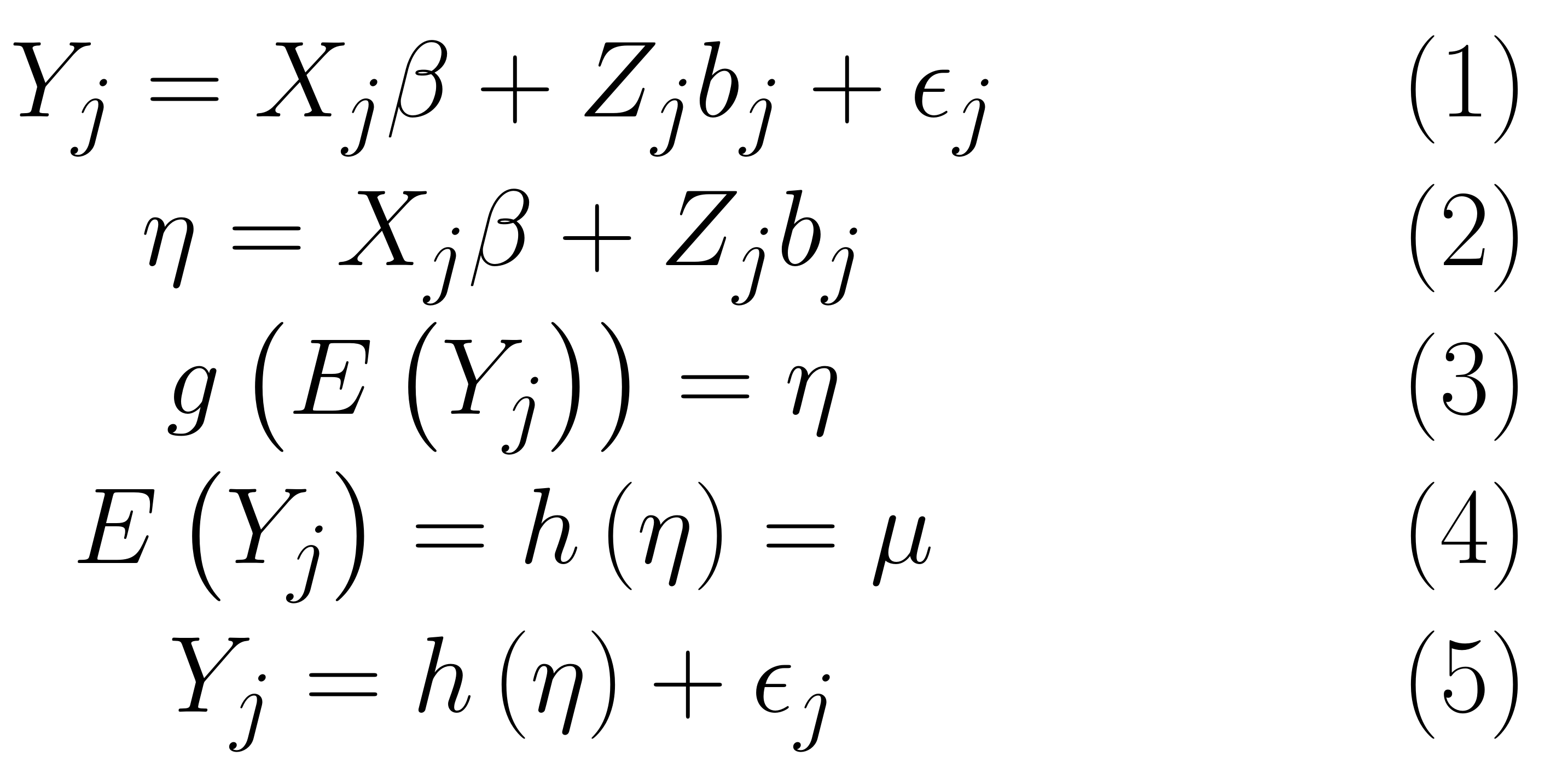
# Linear Mixed Model (LMM)
# Power
- Power is the ability to statistically detect a true effect (i.e. non-zero population effect).
- For simple models (e.g. t-tests, regression) there are closed form equations for generating power.
+ R has routines for these: `power.t.test, power.anova.test`
+ Gpower3
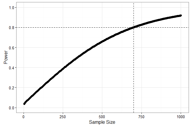
# Power Example
```r
n <- seq(4, 1000, 2)
power <- sapply(seq_along(n), function(i)
power.t.test(n = n[i], delta = .15, sd = 1, type = 'two.sample')$power)
```
# Power for (G)LMM
- Power for more complex models is not as straightforward;
+ particularly with messy real world data.
- There is software for GLMM models to generate power:
+ Optimal Design: <http://hlmsoft.net/od/>
+ MLPowSim: <http://www.bristol.ac.uk/cmm/software/mlpowsim/>
+ Snijders, *Power and Sample Size in Multilevel Linear Models*.
# Power is hard
- In practice, power is hard.
- Need to make many assumptions on data that has not been collected.
+ Therefore, data assumptions made for power computations will likely differ from collected sample.
- A power analysis needs to be flexible, exploratory, and well thought out.
# Power is Fun?
- Three common reasons to do power analysis:
1. Power evidence for grant/planning
2. Post Hoc to explore insignificant results
3. Monte Carlo studies
# `simglm` Overview
- `simglm` aims to simulate (G)LMMs with up to three levels of nesting (aim to add more later).
- Flexible data generation allows:
+ any number of covariates and discrete covariates
+ change distribution of continuous covariates
+ change random distribution
+ unbalanced data
+ missing data
+ serial correlation
# Power with `simglm`
- Power with `simglm` takes on a Monte Carlo approach
+ This can provide a more thorough analysis/understanding of power.
- Always outputs a data frame
+ Useful for plotting
+ Data manipulation
+ etc.
- Serves as a wrapper around data generation process.
# Power Analysis with `simglm`
- Factorial Design:
1. Idenfity factors that influences power
2. Determine number of replications
3. Explore results
- Future Development
1. Add ability for data generation and power model to differ
# Simple Example
- Suppose we wished to generate data for a simple logistic regression.
```r
library(simglm)
fixed <- ~ 1 + act + diff
fixed_param <- c(0.1, 0.5, 0.3)
cov_param <- list(dist_fun = c('rnorm', 'rnorm'),
var_type = c("single", "single"),
opts = list(list(mean = 0, sd = 2),
list(mean = 0, sd = 4)))
n <- 50
temp_single <- sim_glm(fixed = fixed, fixed_param = fixed_param,
cov_param = cov_param,
n = n, data_str = "single")
```
# Output
```r
head(temp_single)
```
```
## X.Intercept. act diff Fbeta logistic sim_data ID
## 1 1 -0.02913722 -0.4430546 -0.04748497 0.4881310 1 1
## 2 1 0.66199364 2.1443743 1.07430910 0.7454155 1 2
## 3 1 1.44621026 -1.1909231 0.46582819 0.6143959 0 3
## 4 1 -0.26011629 3.4395304 1.00180096 0.7314125 0 4
## 5 1 -0.09984213 0.8485436 0.30464201 0.5755769 1 5
## 6 1 -2.72704127 3.3246515 -0.26612517 0.4338586 0 6
```
# Simple Power Analysis
- Suppose we wish to use the same generating model for a power analysis
```r
pow_param <- c('(Intercept)', 'act', 'diff')
alpha <- .01
pow_dist <- "z"
pow_tail <- 2
replicates <- 100
power_out <- sim_pow_glm(fixed = fixed, fixed_param = fixed_param,
cov_param = cov_param,
n = n, data_str = "single",
pow_param = pow_param, alpha = alpha,
pow_dist = pow_dist, pow_tail = pow_tail,
replicates = replicates)
```
# Output
```r
power_out
```
```
## # A tibble: 3 × 6
## var avg_test_stat sd_test_stat power num_reject num_repl
## <fctr> <dbl> <dbl> <dbl> <dbl> <dbl>
## 1 (Intercept) 0.878713 0.6709319 0.01 1 100
## 2 act 2.342617 0.5777646 0.34 34 100
## 3 diff 2.609432 0.5506204 0.56 56 100
```
# Varying Arguments
- Now suppose we wish to vary the following arguments:
- Vary n - 50 vs 150
- vary effect size on diff - .3 vs .45
```r
terms_vary <- list(n = c(50, 150),
fixed_param = list(c(0.1, 0.5, 0.3),
c(0.1, 0.5, 0.45)))
power_out <- sim_pow_glm(fixed = fixed, fixed_param = fixed_param,
cov_param = cov_param,
n = n, data_str = "single",
pow_param = pow_param, alpha = alpha,
pow_dist = pow_dist, pow_tail = pow_tail,
replicates = replicates,
terms_vary = terms_vary)
```
# Output
```r
power_out
```
```
## Source: local data frame [12 x 8]
## Groups: var, n [?]
##
## var n fixed_param avg_test_stat sd_test_stat power
## <fctr> <dbl> <fctr> <dbl> <dbl> <dbl>
## 1 (Intercept) 50 0.1,0.5,0.3 0.7778328 0.5863240 0.00
## 2 (Intercept) 50 0.1,0.5,0.45 0.8364212 0.6377631 0.01
## 3 (Intercept) 150 0.1,0.5,0.3 0.8629973 0.5814426 0.00
## 4 (Intercept) 150 0.1,0.5,0.45 0.9183353 0.6879182 0.01
## 5 act 50 0.1,0.5,0.3 2.4246997 0.6222346 0.44
## 6 act 50 0.1,0.5,0.45 2.2247451 0.6688308 0.34
## 7 act 150 0.1,0.5,0.3 4.3196568 0.6233962 0.99
## 8 act 150 0.1,0.5,0.45 3.9515646 0.6332452 0.97
## 9 diff 50 0.1,0.5,0.3 2.7887204 0.4892985 0.73
## 10 diff 50 0.1,0.5,0.45 3.0747886 0.3988745 0.89
## 11 diff 150 0.1,0.5,0.3 4.7892881 0.5025082 1.00
## 12 diff 150 0.1,0.5,0.45 5.6060130 0.2823105 1.00
## # ... with 2 more variables: num_reject <dbl>, num_repl <dbl>
```
# Move to Mixed Models
- It is simple to move from single level to multilevel or mixed models.
```r
fixed <- ~1 + time + diff + act + time:act
random <- ~1 + time
fixed_param <- c(0, 0.2, 0.1, 0.3, 0.05)
random_param <- list(random_var = c(3, 2), rand_gen = "rnorm")
cov_param <- list(dist_fun = c('rnorm', 'rnorm'),
var_type = c("lvl1", "lvl2"),
opts = list(list(mean = 0, sd = 3),
list(mean = 0, sd = 2)))
n <- 50
p <- 6
data_str <- "long"
temp_long <- sim_glm(fixed = fixed, random = random, fixed_param = fixed_param,
random_param = random_param, cov_param = cov_param,
n = n, p = p, k = NULL, data_str = data_str)
```
# Output
```r
head(temp_long)
```
```
## X.Intercept. time diff act time.act b0 b1
## 1 1 0 -6.76572749 -0.3932853 0.0000000 -1.947485 -2.295427
## 2 1 1 0.15530420 -0.3932853 -0.3932853 -1.947485 -2.295427
## 3 1 2 0.07605058 -0.3932853 -0.7865707 -1.947485 -2.295427
## 4 1 3 -1.11192544 -0.3932853 -1.1798560 -1.947485 -2.295427
## 5 1 4 -4.17141062 -0.3932853 -1.5731413 -1.947485 -2.295427
## 6 1 5 4.77024867 -0.3932853 -1.9664267 -1.947485 -2.295427
## Fbeta randEff logistic prob sim_data withinID clustID
## 1 -0.79455835 -1.947485 -2.742044 6.053757e-02 0 1 1
## 2 0.07788055 -4.242913 -4.165032 1.529175e-02 0 2 1
## 3 0.25029093 -6.538340 -6.288049 1.854935e-03 0 3 1
## 4 0.31182906 -8.833767 -8.521938 1.990136e-04 0 4 1
## 5 0.18621627 -11.129195 -10.942978 1.768142e-05 0 5 1
## 6 1.26071793 -13.424622 -12.163904 5.215325e-06 0 6 1
```
# Doing Power
- Power is also easily extended.
```r
pow_param <- c('time', 'diff', 'act')
alpha <- .01
pow_dist <- "z"
pow_tail <- 2
replicates <- 20
power_out <- sim_pow_glm(fixed = fixed, random = random,
fixed_param = fixed_param,
random_param = random_param, cov_param = cov_param,
k = NULL, n = n, p = p,
data_str = data_str, unbal = FALSE, pow_param = pow_param,
alpha = alpha, pow_dist = pow_dist, pow_tail = pow_tail,
replicates = replicates)
```
# Output
```r
power_out
```
```
## # A tibble: 3 × 6
## var avg_test_stat sd_test_stat power num_reject num_repl
## <fctr> <dbl> <dbl> <dbl> <dbl> <dbl>
## 1 act 12.06197 46.70227 0.20 4 20
## 2 diff 11.89673 45.13827 0.25 5 20
## 3 time 18.78877 79.36869 0.05 1 20
```
# Vary Arguments
- Perhaps our effect size estimate is conservative.
```r
terms_vary <- list(fixed_param = list(c(0, 0.2, 0.1, 0.3, 0.05),
c(0, 0.2, 0.3, 0.3, 0.05)))
power_out <- sim_pow_glm(fixed = fixed, random = random,
fixed_param = fixed_param,
random_param = random_param, cov_param = cov_param,
k = NULL, n = n, p = p,
data_str = data_str, unbal = FALSE, pow_param = pow_param,
alpha = alpha, pow_dist = pow_dist, pow_tail = pow_tail,
replicates = replicates,
terms_vary = terms_vary)
```
# Output
```r
power_out
```
```
## Source: local data frame [6 x 7]
## Groups: var [?]
##
## var fixed_param avg_test_stat sd_test_stat power num_reject
## <fctr> <fctr> <dbl> <dbl> <dbl> <dbl>
## 1 act 0,0.2,0.1,0.3,0.05 1.1914255 0.8114762 0.10 2
## 2 act 0,0.2,0.3,0.3,0.05 22.9059014 96.3531136 0.15 3
## 3 diff 0,0.2,0.1,0.3,0.05 1.3071639 0.8681348 0.05 1
## 4 diff 0,0.2,0.3,0.3,0.05 17.4774138 62.2814403 0.95 19
## 5 time 0,0.2,0.1,0.3,0.05 0.9281452 0.7670600 0.05 1
## 6 time 0,0.2,0.3,0.3,0.05 12.1678311 49.9607401 0.05 1
## # ... with 1 more variables: num_repl <dbl>
```
# Shiny App
- Note: This app currently looks nice, but is utterly broken!
```r
shiny::runGitHub('simglm', username = 'lebebr01', subdir = 'inst/shiny_examples/demo')
```
or
```r
devtools::install_github('lebebr01/simglm')
library(simglm)
run_shiny()
```
- Must have following packages installed: `simglm, shiny, shinydashboard, ggplot2, lme4, DT`.
# `simglm` timeline
- Aim to have this package submitted to CRAN by the end of March.
- Fix Shiny application.
- For now look for the package on GitHub <http://github.com/lebebr01/simglm>
# Questions?
- Twitter: @blebeau11
- Website: <http://brandonlebeau.org>
- Slides: <http://brandonlebeau.org/2017/02/24/csp2017.html>
- GitHub: <http://github.com/lebebr01/simglm>