<h1>Tidy Meta-Analytic Data</h1>
<h2>Brandon LeBeau & Ariel M. Aloe</h2>
<h3>University of Iowa</h3>
# Rationale
- Data entry is an important component for quantitative studies
+ Often neglected in courses
- Messy data can make data manipulation much more difficult
+ Substantial time could be lost due to poor data entry procedures
- Strong data entry procedures are particularly important in evidence synthesis
# Rationale 2
- Data Organization in Spreadsheets - Broman and Woo (2018), *The American Statistician*, https://doi.org/10.1080/00031305.2017.1375989
- Tidy Data - Wickham (2014), *Journal of Statistical Software*, https://www.jstatsoft.org/index.php/jss/article/view/v059i10
- Nine simple ways to make it easier to (re)use your data - White et al., (2013), https://ojs.library.queensu.ca/index.php/IEE/article/view/4608
# Tidy Meta Analytic Data
- A series of data entry rules
- Promotes more consistent evidence synthesis data
- Promotes reproducible analyses (See Reproducible Analyses in Education Research by LeBeau, Ellison, Aloe (2021) in Review of Research in Education).
- Promotes reusable analyses across evidence synthesis projects
- Facilitates a split-apply-combine data analysis framework (Wickham, 2011; https://www.jstatsoft.org/v40/i01/)
# Data Entry Rules
- These rules are mostly agnostic to data storage mode/program
+ Text based (csv, tsv, etc.)
+ SQL databases of all types
+ Excel (but please avoid)
- Rows should be the unit of analysis
- Columns are attributes/characteristics about a unit of analysis
- Data should be rectangular
# Column Rules
1. Avoid placing attributes/characteristics in column names
2. Do not use spaces in names
3. Columns should contain one attribute/characteristic
4. Use one row for column names
5. Ensure appropriate ID columns
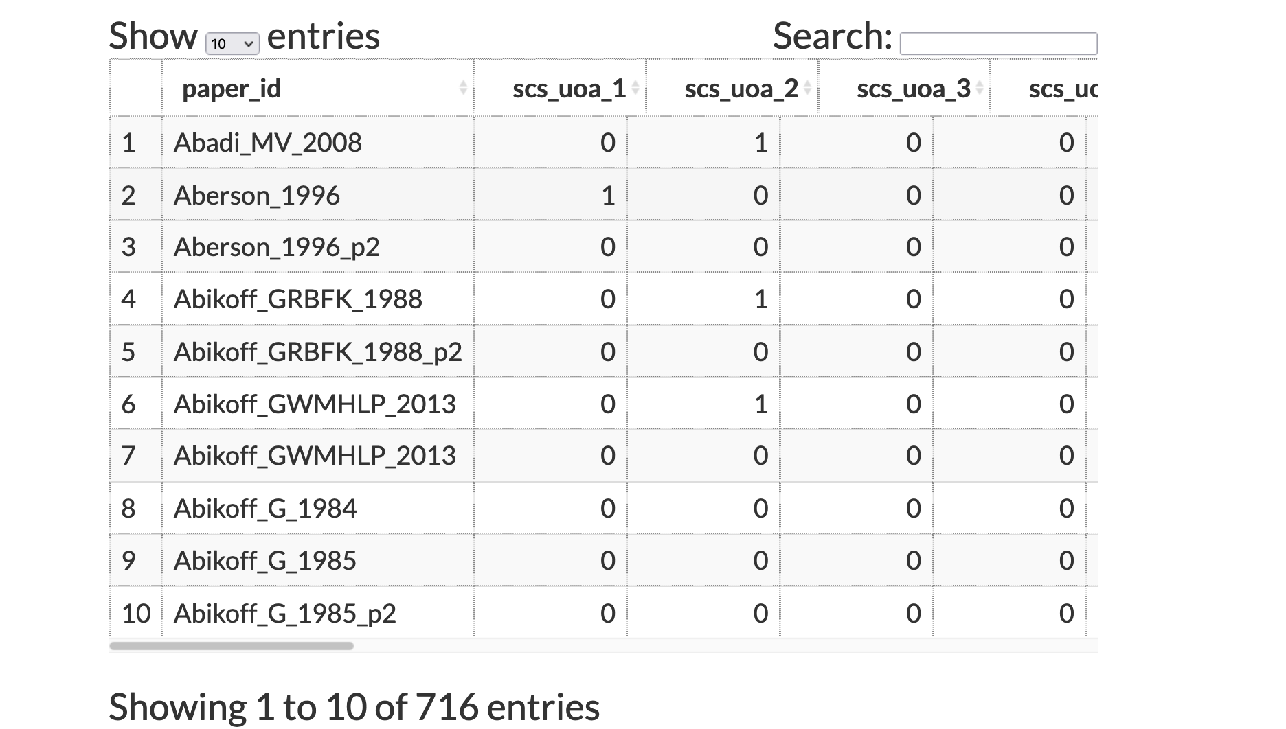
# Column Example(s)
# Row Rules
1. Have deliberate missing data codes:
+ Using -99, 99, -9999, N/A are problematic
+ NA is a good option
2. No calculations in the data file
3. Use ISO 8601 standard for dates YYYY-MM-DD (https://xkcd.com/1179/)
+ Particularly needed when using Excel
4. Don't use highlighting as data
+ TRUE/FALSE attributes can be helpful here
# Date Conversion Excel
# Highlighting Cells
# Split-Apply-Combine
- Process of splitting a hard task into smaller manageable tasks
- This framework is particularly powerful in functional programming languages, like R, Python, Julia, Scala, Mathematica, Javascript, etc.
- Split-Apply-Combine in Data Analysis
+ Split observations into similar type
+ Apply a function (ie, often a computation)
+ Combine function results across observations
# Synthesis of Correlation Matrices
- One particular way to implement of tidy meta analytic data is the synthesis of correlation matrices.
- See *Meta-Analysis of Correlations, Correlation Matrices, and Their Functions* by Becker, Aloe, Cheung (2020) in Handbook of Meta-Analysis
- We will use an R package developed in tandem with this chapter, `metaRmat`.
# Install `metaRmat`
```r
remotes::install_github("lebebr01/metaRmat")
```
```r
library(metaRmat)
```
# Correlation Data Example
```r
becker09[, 1:6]
```
```
## ID N Team Cognitive_Performance Somatic_Performance
## 1 1 142 I -0.55 -0.48
## 2 3 37 I 0.53 -0.12
## 3 6 16 T 0.44 0.46
## 4 10 14 I -0.39 -0.17
## 5 17 45 I 0.10 0.31
## 6 22 100 I 0.23 0.08
## 7 26 51 T -0.52 -0.43
## 8 28 128 T 0.14 0.02
## 9 36 70 T -0.01 -0.16
## 10 38 30 I -0.27 -0.13
## Selfconfidence_Performance
## 1 0.66
## 2 0.03
## 3 NA
## 4 0.19
## 5 -0.17
## 6 0.51
## 7 0.16
## 8 0.13
## 9 0.42
## 10 0.15
```
# Split Correlation Matrices
```r
becker09_list <- df_to_corr(becker09,
variables =
c('Cognitive_Performance',
'Somatic_Performance',
'Selfconfidence_Performance',
'Somatic_Cognitive',
'Selfconfidence_Cognitive',
'Selfconfidence_Somatic'),
ID = 'ID')
```
# View Split Correlation Matrices
```r
becker09_list[1:3]
```
```
## $`1`
## Performance Cognitive Somatic Selfconfidence
## Performance 1.00 -0.55 -0.48 0.66
## Cognitive -0.55 1.00 0.47 -0.38
## Somatic -0.48 0.47 1.00 -0.46
## Selfconfidence 0.66 -0.38 -0.46 1.00
##
## $`3`
## Performance Cognitive Somatic Selfconfidence
## Performance 1.00 0.53 -0.12 0.03
## Cognitive 0.53 1.00 0.52 -0.48
## Somatic -0.12 0.52 1.00 -0.40
## Selfconfidence 0.03 -0.48 -0.40 1.00
##
## $`6`
## Performance Cognitive Somatic Selfconfidence
## Performance 1.00 0.44 0.46 NA
## Cognitive 0.44 1.00 0.67 NA
## Somatic 0.46 0.67 1.00 NA
## Selfconfidence NA NA NA 1
```
# Correlations as Tidy Meta Analytic Data
```r
input_metafor <- prep_data(becker09,
becker09$N,
type = 'weighted', missing = FALSE,
variable_names =
c('Cognitive_Performance',
'Somatic_Performance',
'Selfconfidence_Performance',
'Somatic_Cognitive',
'Selfconfidence_Cognitive',
'Selfconfidence_Somatic'),
ID = 'ID')
```
# View Tidy Meta Analytic Correlations
```r
head(input_metafor$data, n = 15)
```
```
## Variable1 Variable2 yi outcome study
## 1 Performance Cognitive -0.55 1 1
## 2 Performance Somatic -0.48 2 1
## 3 Performance Selfconfidence 0.66 3 1
## 4 Cognitive Somatic 0.47 4 1
## 5 Cognitive Selfconfidence -0.38 5 1
## 6 Somatic Selfconfidence -0.46 6 1
## 7 Performance Cognitive 0.53 1 2
## 8 Performance Somatic -0.12 2 2
## 9 Performance Selfconfidence 0.03 3 2
## 10 Cognitive Somatic 0.52 4 2
## 11 Cognitive Selfconfidence -0.48 5 2
## 12 Somatic Selfconfidence -0.40 6 2
## 13 Performance Cognitive 0.44 1 3
## 14 Performance Somatic 0.46 2 3
## 15 Performance Selfconfidence NA 3 3
```
# Fit a random effects meta analytic model
```r
random_model <- fit_model(data = input_metafor, effect_size = 'yi',
var_cor = 'V', moderators = ~ -1 + factor(outcome),
random_params = ~ factor(outcome) | factor(study))
```
```r
round(random_model$tau2, 3) # between studies variance
```
```
## [1] 0.126 0.060 0.062 0.002 0.011 0.006
```
```r
round(random_model$b, 3) # random effect estimate
```
```
## [,1]
## factor(outcome)1 -0.034
## factor(outcome)2 -0.071
## factor(outcome)3 0.233
## factor(outcome)4 0.544
## factor(outcome)5 -0.453
## factor(outcome)6 -0.397
```
# Average correlation matrix
```r
model_out_random <- extract_model(random_model,
variable_names = c('Cognitive_Performance',
'Somatic_Performance',
'Selfconfidence_Performance',
'Somatic_Cognitive',
'Selfconfidence_Cognitive',
'Selfconfidence_Somatic'))
round(model_out_random$beta_matrix, 3)
```
```
## Performance Cognitive Somatic Selfconfidence
## Performance 1.000 -0.034 -0.071 0.233
## Cognitive -0.034 1.000 0.544 -0.453
## Somatic -0.071 0.544 1.000 -0.397
## Selfconfidence 0.233 -0.453 -0.397 1.000
```
# Fit path model
```r
model <- "## Regression paths
Performance ~ Cognitive + Somatic + Selfconfidence
Selfconfidence ~ Cognitive + Somatic
"
path_output <- path_model(data = model_out_random, model = model,
num_obs = sum(becker09$N))
```
# Extract some results
```r
path_output$parameter_estimates
```
```
## [[1]]
## predictor outcome estimate
## Cognitive -> Performance Cognitive Performance 0.09757045
## Somatic -> Performance Somatic Performance -0.01663048
## Selfconfidence -> Performance Selfconfidence Performance 0.27041818
##
## [[2]]
## predictor outcome estimate
## Cognitive -> Selfconfidence Cognitive Selfconfidence -0.3359884
## Somatic -> Selfconfidence Somatic Selfconfidence -0.2146362
```
# Summary
- Be mindful and plan for data entry - this is hard!
- Do not assume that data entry will "take care of itself"
- Think "long" instead of wide
- Ensure attributes contain one piece of information
- Ensure attributes are named well, but do not contain information directly
- Use text based or database systems rather than Excel
# Connect
- slides: https://brandonlebeau.org/slides/canam2021/
- twitter: blebeau11