remotes::install_github('lebebr01/simglm')simglm v0.9.22: Propensity Score Simulation
R
simglm
simulation
propensity scores
I haven’t written about my simglm package in a while. Behind the scenes, numerous changes have been made to enhance the package. The current CRAN version is significantly behind, but my goal is to submit the most recent version to CRAN soon, once I finalize the details for my upcoming book on simulation and power analysis with R, published by CRC Press.
One of the final implementations required for this book is conducting a simulation and power analysis for propensity scores. Propensity scores can be helpful to adjust for observed/collected data when randomization was not done or was not feasible. Propensity scores are used to estimate the probability that a data unit is included in the treatment condition using a function of observed data attributes. This procedure can help adjust, statistically, for differences in data attributes across the treatment and control groups.
For example, we would not be able to assign people to smoke randomly, so instead, we need to collect information from people who already smoke compared to those who do not smoke. Due to people self-selecting to smoke or not, these groups would likely differ, which would make the impact of any potential health outcomes vary due to baseline differences. Propensity scores help balance the groups based on observed characteristics before any intervention.
With these simulation tools, you can now not only model realistic quasi-experimental data but also assess how much sample size you need to detect treatment effects reliably.
simglm simulation for propensity scores
In the most recent version of the simglm package on GitHub, support for simulating data using propensity scores is now available. The simulation procedure takes a two-step approach.
- Step 1: Simulate the group membership using logistic regression as a function of some data attributes.
- Step 2: Simulate any additional attributes and incorporate the group membership from step 1. Step 1 is essential, as now the group membership would not be randomly assigned; instead, whether someone is simulated to be in the treatment group would depend on the attributes specified in step 1.
First, ensure that you install the updated simglm package from GitHub, along with the remotes package.
Here is an example of how step 1 can be specified within the simglm package. A new named element to the simulation arguments, called “propensity,” specifies the components used to generate the group membership. The required elements in here are similar to those from the Tidy Simulation vignette. It is essential to define the attributes that distinguish a person’s inclusion in the treatment or control group using the model formula. In the example below, age and socio-economic status (SES) are the two data attributes being used to define who belongs in the treatment or control group. The regression weights argument specifies the relationship between being in the treatment or control group.
Finally, with the outcome_type = 'binary' specification, logistic regression is used to estimate the propensity scores and generate the probability of being in the treatment or control group.
library(simglm)

sim_arguments <- list(
    propensity = list(
        formula = trt ~ 1 + age + ses,
        fixed = list(age = list(var_type = 'ordinal',
                         levels = -7:7),
                     ses = list(var_type = 'continuous',
                         mean = 0, sd = 5)),
        sample_size = 250,
        error = list(variance = 5),
        reg_weights = c(2, 0.3, 0.15),
        outcome_type = 'binary'
    )
)

prop_data <- simulate_propensity(sim_arguments)
Once we simulate the propensity data, we can visualize the balance between the treatment and control groups by the two data attributes, age and SES.
Age balance
First, examining the balance by age reveals that individuals in the treatment group tend to be older than those in the control group. These are differences that may be meaningful and impact the estimation of the actual treatment effect.
library(ggformula)

prop_data |>
    gf_density(~ age, fill = ~factor(trt)) |>
    gf_labs(fill = "Treatment")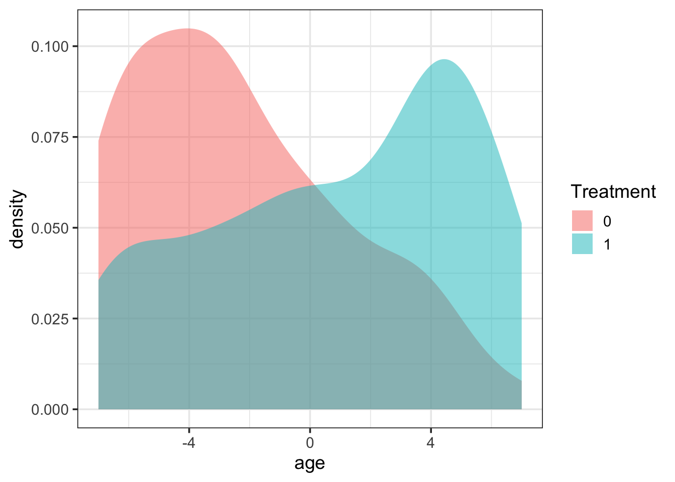
SES balance
The SES balance is again in the positive direction, with the treatment group coming from slightly higher SES backgrounds compared to those in the control group. Without adjusting for this, the treatment effect would likely be biased.
prop_data |>
    gf_density(~ ses, fill = ~factor(trt)) |>
    gf_labs(fill = "Treatment")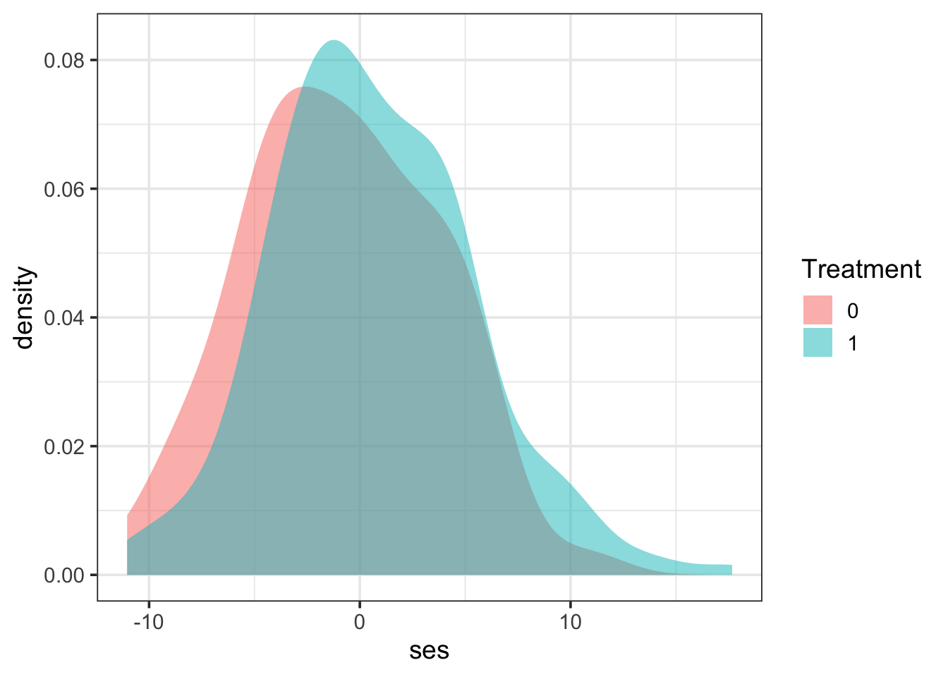
Full data simulation with propensity scores
Below is an example that incorporates a full data simulation with the treatment group generated from the propensity score model (i.e., logistic regression). In this hypothetical example, we aim to model student achievement as a function of motivation, the treatment group (generated via propensity scores), age, and SES. The simulated treatment effect was specified as 1.2. This effect was generated not to be a standardized effect size here, as this is entirely hypothetical; however, it is often easiest to specify effects as standardized effect sizes.
sim_arguments <- list(
    formula = achievement ~ 1 + motivation + trt + age + ses,
    fixed = list(
        motivation = list(var_type = 'continuous',
                           mean = 0, sd = 20)
    ),
    sample_size = 250,
    error = list(variance = 10),
    reg_weights = c(50, 0.4, 1.2, 0.1, 0.25),
    propensity = list(
        formula = trt ~ 1 + age + ses,
        fixed = list(age = list(var_type = 'ordinal',
                         levels = -7:7),
                     ses = list(var_type = 'continuous',
                         mean = 0, sd = 5)),
        sample_size = 250,
        error = list(variance = 5),
        reg_weights = c(2, 0.3, -0.5),
        outcome_type = 'binary'
    )
)
sim_data <- simulate_fixed(data = NULL, sim_args = sim_arguments) |>
    simulate_error(sim_args = sim_arguments) |>
    generate_response(sim_arguments)

DT::datatable(sim_data)
The simulation process uses the treatment, age, and SES data generated from the propensity score process. That is, these attributes are not regenerated in the process, but are simulated first, then any additional fixed effects are simulated to work through the simulation pipeline.
Estimate propensity models with simglm
The model estimation process is done similarly to the simulation process. Two models are estimated via a two-step process.
- Step 1: A propensity score model is estimated to estimate the probability of being in the treatment group. This is controlled via the
propensity_modelsimulation arguments below. - Step 2: A full model is estimated, specified via the
model_fitsimulation arguments. The propensity scores can be included in three different ways via the “propensity_type” simulation argument:- covariate: The propensity score probabilities are included as a covariate in the final model.
- ipw: Inverse propensity score weighting is used and passed to the weights argument of the model.
- sbw: Stabilized propensity score weighting is used and passed to the weights arguments of the model. The stabilized weights use the mean of the propensity scores instead of 1, which can help limit weights that are excessively large or small.
Covariate-adjusted model
The covariate-adjusted model includes the propensity score as a covariate in the final model via the propensity_type = 'covariate' argument.
sim_arguments <- list(
    formula = achievement ~ 1 + motivation + trt + age + ses,
    fixed = list(
        motivation = list(var_type = 'continuous',
                           mean = 0, sd = 20)
    ),
    sample_size = 1000,
    error = list(variance = 10),
    reg_weights = c(50, 0.4, 1.2, 0.1, 0.25),
    propensity = list(
        formula = trt ~ 1 + age + ses,
        fixed = list(age = list(var_type = 'ordinal',
                         levels = -7:7),
                     ses = list(var_type = 'continuous',
                         mean = 0, sd = 5)),
        sample_size = 1000,
        error = list(variance = 5),
        reg_weights = c(2, 0.3, -0.5),
        outcome_type = 'binary'
    ),
    model_fit = list(formula = achievement ~ 1 + motivation + trt + age + ses,
                   model_function = 'lm'),
    propensity_model = list(
        formula = trt ~ 1 + age + ses,
        propensity_type = 'covariate'
    )
)
simulate_fixed(data = NULL, sim_args = sim_arguments) |>
  simulate_error(sim_args = sim_arguments) |>
  generate_response(sim_arguments)|>
  fit_propensity(sim_arguments) |>
  model_fit(sim_arguments) |>
  extract_coefficients()
# A tibble: 6 × 5
term estimate std.error statistic p.value
<chr> <dbl> <dbl> <dbl> <dbl>
1 (Intercept) 51.1 0.912 56.0 6.71e-310
2 motivation 0.402 0.00480 83.7 0
3 trt 1.34 0.257 5.21 2.30e- 7
4 age 0.145 0.0383 3.79 1.58e- 4
5 ses 0.208 0.0582 3.57 3.75e- 4
6 propensity -1.75 1.31 -1.34 1.80e- 1Inverse Propensity Score Weighting
To specify inverse propensity score weighting, propensity_type = 'ipw' is specified. Note that the propensity scores are no longer included as a covariate.
sim_arguments <- list(
    formula = achievement ~ 1 + motivation + trt + age + ses,
    fixed = list(
        motivation = list(var_type = 'continuous',
                           mean = 0, sd = 20)
    ),
    sample_size = 1000,
    error = list(variance = 10),
    reg_weights = c(50, 0.4, 1.2, 0.1, 0.25),
    propensity = list(
        formula = trt ~ 1 + age + ses,
        fixed = list(age = list(var_type = 'ordinal',
                         levels = -7:7),
                     ses = list(var_type = 'continuous',
                         mean = 0, sd = 5)),
        sample_size = 1000,
        error = list(variance = 5),
        reg_weights = c(2, 0.3, -0.5),
        outcome_type = 'binary'
    ),
    propensity_model = list(
        formula = trt ~ 1 + age + ses,
        propensity_type = 'ipw'
    )
)
simulate_fixed(data = NULL, sim_args = sim_arguments) |>
  simulate_error(sim_args = sim_arguments) |>
  generate_response(sim_arguments)|>
  fit_propensity(sim_arguments) |>
  model_fit(sim_arguments) |>
  extract_coefficients()
# A tibble: 5 × 5
term estimate std.error statistic p.value
<chr> <dbl> <dbl> <dbl> <dbl>
1 (Intercept) 49.9 0.203 246. 0
2 motivation 0.406 0.00510 79.7 0
3 trt 1.12 0.253 4.43 1.03e- 5
4 age 0.129 0.0241 5.35 1.07e- 7
5 ses 0.272 0.0226 12.0 3.50e-31Stabilized Propensity Score Weighting
To specify stabilized propensity score weighting, propensity_type = 'sbw' is specified. Note that the propensity scores are no longer included as a covariate.
sim_arguments <- list(
    formula = achievement ~ 1 + motivation + trt + age + ses,
    fixed = list(
        motivation = list(var_type = 'continuous',
                           mean = 0, sd = 20)
    ),
    sample_size = 1000,
    error = list(variance = 10),
    reg_weights = c(50, 0.4, 1.2, 0.1, 0.25),
    propensity = list(
        formula = trt ~ 1 + age + ses,
        fixed = list(age = list(var_type = 'ordinal',
                         levels = -7:7),
                     ses = list(var_type = 'continuous',
                         mean = 0, sd = 5)),
        sample_size = 1000,
        error = list(variance = 5),
        reg_weights = c(2, 0.3, -0.5),
        outcome_type = 'binary'
    ),
    propensity_model = list(
        formula = trt ~ 1 + age + ses,
        propensity_type = 'sbw'
    )
)
simulate_fixed(data = NULL, sim_args = sim_arguments) |>
  simulate_error(sim_args = sim_arguments) |>
  generate_response(sim_arguments)|>
  fit_propensity(sim_arguments) |>
  model_fit(sim_arguments) |>
  extract_coefficients()
# A tibble: 5 × 5
term estimate std.error statistic p.value
<chr> <dbl> <dbl> <dbl> <dbl>
1 (Intercept) 50.2 0.206 244. 0
2 motivation 0.402 0.00528 76.1 0
3 trt 1.03 0.259 3.99 6.99e- 5
4 age 0.0942 0.0248 3.80 1.54e- 4
5 ses 0.239 0.0232 10.3 1.35e-23Each of these approaches has the potential to produce a more balanced comparison between the treatment and control groups for observed data attributes. The primary limitation of propensity scores compared to actual random assignment is that they cannot adjust for any differences in data attributes that are unobserved. True random assignment can help ensure that the treatment and control groups are balanced with respect to observed and unobserved data attributes. Even with this limitation, propensity scores are preferable to doing nothing when random assignment is not possible or cannot be performed.
Next Steps
The next step is to ensure that these propensity score simulation and model estimation steps are included in the broader functions to perform replications. This will enable the estimation of power for planning a study that aims to implement propensity scores.
If you work with non-randomized designs, simglm can now help you simulate realistic scenarios, test different adjustment methods, and plan studies with more confidence.