Overview

1. Power
2. simglm package
3. Shiny Demo

Power

• Power is the ability to statistically detect a true effect (i.e. non-zero population effect).
• For simple models (e.g. t-tests, regression) there are closed form equations for generating power.
  • R has routines for these: power.t.test, power.anova.test
  • Gpower3

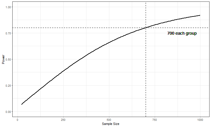
Power Example

n <- seq(20, 1000, 5)
power <- sapply(seq_along(n), function(i) 
  power.t.test(n = n[i], delta = .15, sd = 1, type = 'two.sample')$power)

Power for (G)LMM

• Power for more complex models is not as straightforward;
  • particularly with messy real world data.
• There is software for GLMM models to generate power
  • Optimal Design: http://hlmsoft.net/od/
  • MLPowSim: http://www.bristol.ac.uk/cmm/software/mlpowsim/
  • Snijders, Power and Sample Size in Multilevel Linear Models.
  • Moerbeek & Teerenstra, Power Analysis of Trials with Multilevel Data.

Power is hard

• In practice, power is hard.
• Need to make many assumptions on data that has not been collected.
  • Therefore, data assumptions made for power computations will likely differ from collected sample.
• A power analysis needs to be flexible, exploratory, and well thought out.

Why do power?

• Three common reasons to do power analysis:
  1. Power evidence for grant/planning
  2. Post Hoc to explore insignificant results
  3. Monte Carlo studies

simglm Features

• Longitudinal data simulation
• Three levels of nesting
• Specification of distribution of random components (random effects and random error)
• Specification of serial correlation
• Specification of the number of variables
  • Ability to add time-varying covariates
  • Specify the mean and variance of fixed covariate variables
  • Factor variable simulation
  • Ordinal variable simulation

simglm Features Continued

• Power by simulation
  • Vary parameters for a factorial simulation design.
  • Can vary model fitted to the data to misspecify directly.
• Simulation of missing data
• Include other distributions for covariate simulation.
• Continuous, Logistic (dichotomous), and Poisson (count) outcome variables.

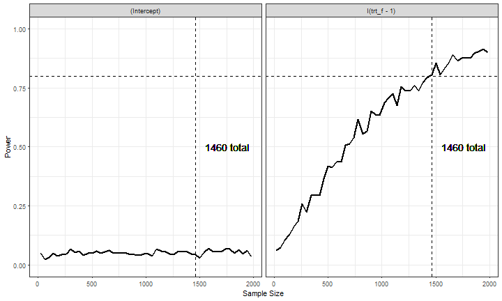
Replicate with simglm

• Note this code uses the development version on GitHub

library(simglm)
fixed <- ~ 1 + trt_f
fixed_param <- c(0, 0.15)
fact_vars <- list(numlevels = 2, var_type = 'single', 
                  opts = list(list(replace = TRUE)))
n <- NULL
error_var <- 1
with_err_gen <- 'rnorm'
pow_param <- c('(Intercept)', 'I(trt_f - 1)')
alpha <- .05
pow_dist <- "t"
pow_tail <- 2
replicates <- 500
terms_vary <- list(n = seq(20, 2000, 40))
power_out <- sim_pow(fixed = fixed, fixed_param = fixed_param, cov_param = NULL,
                     n = n, error_var = error_var, with_err_gen = with_err_gen,
                     fact_vars = fact_vars,
                     data_str = "single", pow_param = pow_param, alpha = alpha,
                     pow_dist = pow_dist, pow_tail = pow_tail, 
                     replicates = replicates, terms_vary = terms_vary, 
                     raw_power = FALSE, lm_fit_mod = sim_data ~ I(trt_f - 1))

Plot Results

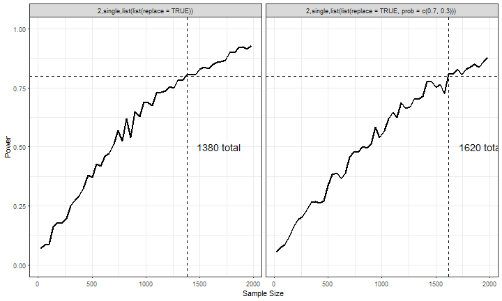
More Realistic?

terms_vary <- list(n = seq(20, 2000, 40),
                   fact_vars = list(list(numlevels = 2, var_type = 'single', 
                                      opts = list(list(replace = TRUE))),
                                    list(numlevels = 2, var_type = 'single', 
                                      opts = list(list(replace = TRUE, 
                                                       prob = c(.7, .3))))))
pow_param <- c('I(trt_f - 1)')
power_out <- sim_pow(fixed = fixed, fixed_param = fixed_param, cov_param = NULL,
                     n = n, error_var = error_var, with_err_gen = with_err_gen,
                     fact_vars = fact_vars,
                     data_str = "single", pow_param = pow_param, alpha = alpha,
                     pow_dist = pow_dist, pow_tail = pow_tail, 
                     replicates = replicates, terms_vary = terms_vary, 
                     raw_power = FALSE, lm_fit_mod = sim_data ~ I(trt_f - 1))

Results

Shiny Demo

• Once the package is installed, can run the Shiny app locally.

run_shiny()

Connect

• Twitter: @blebeau11
• Website: https://brandonlebeau.org
• Slides: https://brandonlebeau.org/slides/jsm2017.html
• GitHub: http://github.com/lebebr01/simglm