Research Problem

• IRT models specified as linear mixed models are not new (e.g., Adams, Wilson, & Wu, 1997; Kamata, 2001; Mellenbergh, 1994; Rijmen et al., 2003).
• Some have discussed evaluating DIF in these frameworks too (e.g., Noorgate and De Boeck, 2005).
• To our knowledge, these methods have not been explored to which the extent they properly link scores.

Heterotypic Continuity

• We approach this research primarily from a psychological measurement lens, where heterotypic continuity is often of concern.
• Heterotypic Continuity occurs when the same psychological reasons underlie different behaviors at different ages—the same construct looks different across development (Petersen, Choe & LeBeau, 2020).
• Examples: Externalizing Problems (Petersen & LeBeau, 2020; Petersen & LeBeau, 2021)

Limitations of current linking

• Item parameter estimates treated as known parameters for linking.
  • Problematic in small samples
• Does not account for any clustering in the data collection design
• Current software for linking is cumbersome to use.
  • Limits use for applied researchers

Bayesian Generalized Linear Mixed Model

Focusing on dichotomous items, we could define a 2pl IRT model within a linear mixed model:

$$ P(y = 1) = logistic(\alpha{i}(b{p} + \gamma_{i})) $$

• $\alpha_{i}$ is item specific discrimination
• $b_{p}$ is a random person effect, often called theta or ability
• $\gamma_{i}$ is an item easiness term

Adding Attributes

Attributes can be added as item, person, or both item and person attributes.

Example:

$$ P(y = 1) = logistic(\alpha{i}(b{p} + \gamma{i} + X{jpi} \beta_{j})) $$

• $X_{jpi}$ is a design matrix.
• $\beta_{j}$ are a set of $J$ regression coefficients.

Specific Example - 3 time points

Example

$$ P(y = 1) = logistic(\alpha{i}(b{p} + \gamma{i} + \beta{1} time{2} + \beta{2} time_{3})) $$

• $time_{2}$ is a dummy attribute, 1 = time 2, 0 = otherwise
• $time_{3}$ is a dummy attribute, 1 = time 3, 0 = otherwise

Simulation Conditions

• Sample size fixed at 1000
• 3 time points
• Number of items fixed at 20 for each time point
• 10 common items (40 total items, 10 in common, 10 unique across 3 time points)
• Change in common easiness: -0.5, 0, 0.5

Data Generation

• Data were generated by randomly generating 1000 person parameters (ability/theta)
• Item parameter were randomly generated for all unique items (30 items)
• Common item parameters at each time point were shifted based on the change in common easiness.

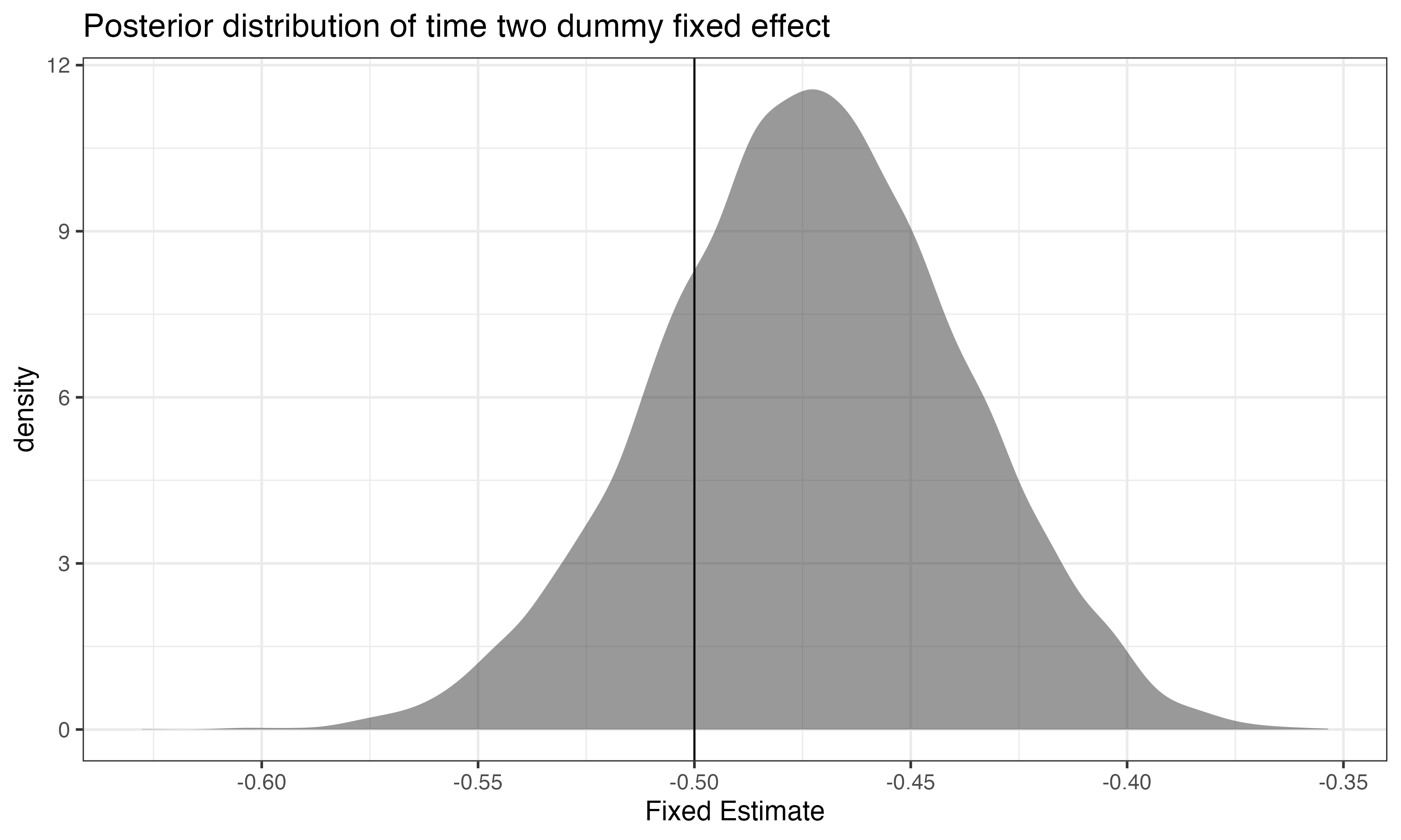
Fixed Effect Results - Time 2

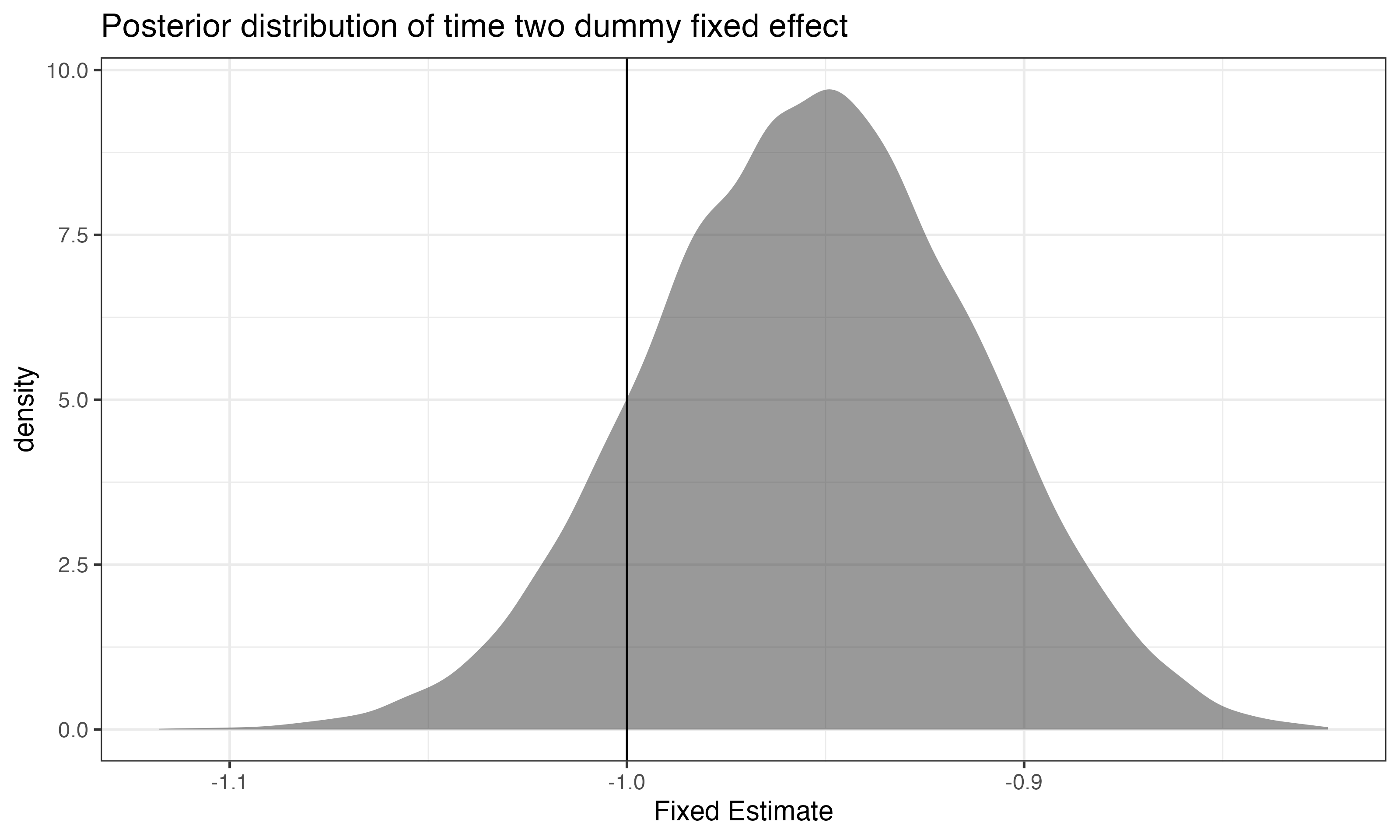
Fixed Effect Results - Time 3

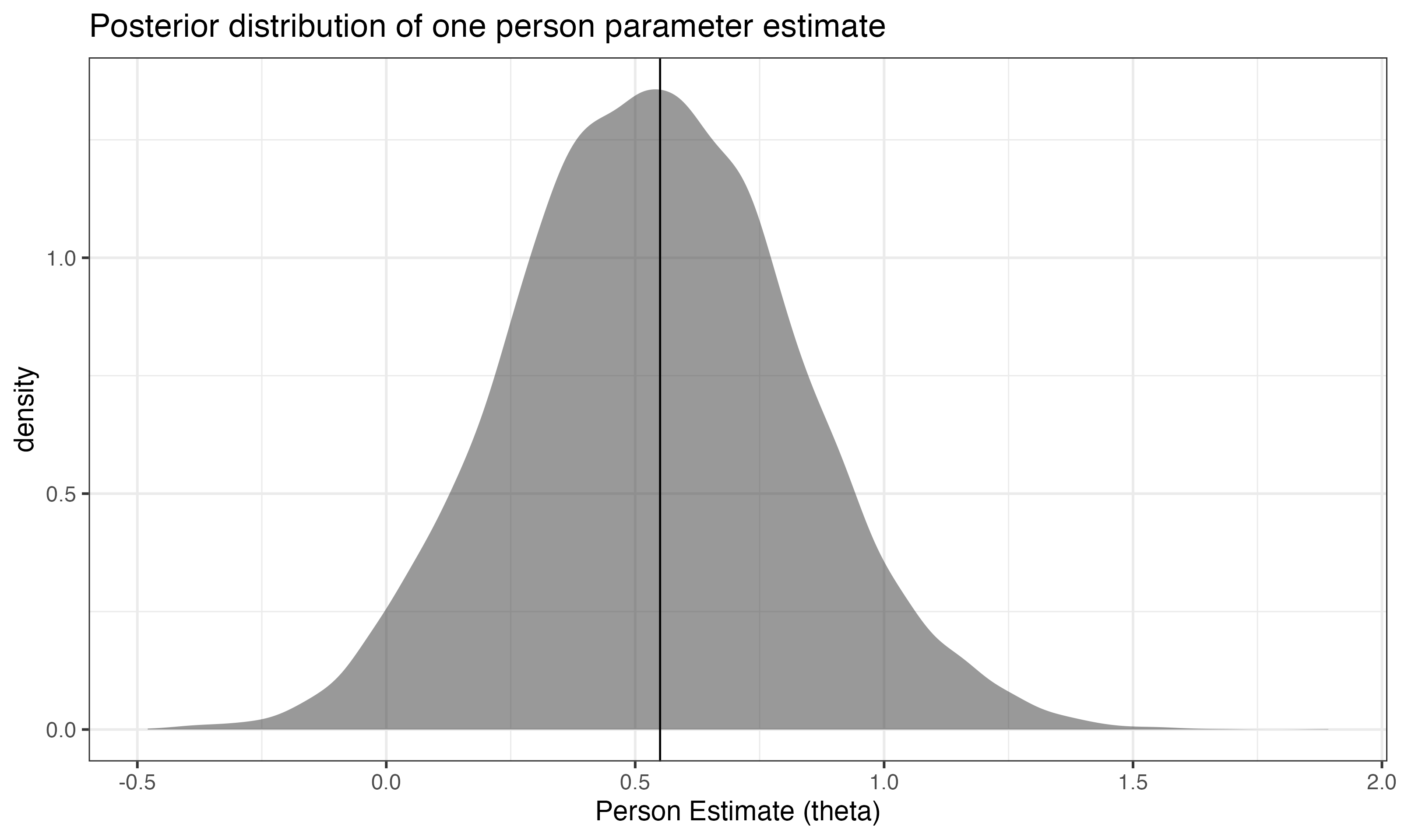
Recovering Ability

Concluding Remarks

• Fitting IRT models as mixed models is highly flexible.
• Preliminary evidence suggests adequate recovery of parameters.
• May work in small samples due to ability to impose prior information

Future Work

• Vary more data conditions to evaluate ability to link across different situations
  • Non-linear change across time
  • More time points
  • Smaller sample size
• Evaluate more complex model to allow variance of person parameters to change over time

Get in Touch

• webpage: https://brandonlebeau.org/
• twitter: @blebeau11
• GitHub: lebebr01
• LinkedIn: blebeau11
• slides: https://brandonlebeau.org/slides/ncme-2023