remotes::install_github('lebebr01/simglm')simglm v0.9.23: Propensity Score Modeling
R
simglm
modeling
propensity scores
Building on last week’s post about propensity score simulation, the simglm package has been extended to now allow for the estimation of power in addition to the propensity score simulations. Recall, propensity scores can be helpful for causal inference with intact groups, when random assignment was either not possible or not done. This allows for the estimation of power under all three supported propensity score methods:
- Covariate adjustment
- Inverse propensity score weighting
- Stabilized propensity score weighting
One nice feature is that no additional simulation arguments are needed to handle the model fitting and replication procedures. These pass directly from the previous functionality handled from within the package. One small adjustment was made internally to allow for the inclusion of the propensity score covariate when that option is specified. Since this term is not usually of substantive value, it can be filtered out from the final output as well.
If you haven’t already, remember to first install the simglm package from GitHub.
Fitting a covariate adjusted model.
The below code does the following steps:
- Simulates the data with the propensity model. That is, the treatment attribute is simulated as a function of age and SES so that those that are older and higher SES are more likely to be in the treatment group.
- Simulates the full model to generate scores for student achievement.
- Fit propensity score model to the simulated data.
- Fit the final model, with the estimated propensity scores included as a covariate, and store model estimates.
- Repeat steps 1–4 for 500 replications (illustrative only; use more in practice).
To fit the propensity score adjusted covariate model, propensity_type = 'covariate' is added to the propensity model simulation arguments.
library(simglm)

sim_arguments <- list(
    formula = achievement ~ 1 + motivation + trt + age + ses,
    fixed = list(
        motivation = list(var_type = 'continuous',
                           mean = 0, sd = 20)
    ),
    sample_size = 1000,
    error = list(variance = 10),
    reg_weights = c(50, 0.4, 1.2, 0.1, 0.25),
    propensity = list(
        formula = trt ~ 1 + age + ses,
        fixed = list(age = list(var_type = 'ordinal',
                         levels = -7:7),
                     ses = list(var_type = 'continuous',
                         mean = 0, sd = 5)),
        sample_size = 1000,
        error = list(variance = 5),
        reg_weights = c(2, 0.3, -0.5),
        outcome_type = 'binary'
    ),
    model_fit = list(formula = achievement ~ 1 + motivation + trt + age + ses,
                   model_function = 'lm'),
    propensity_model = list(
        formula = trt ~ 1 + age + ses,
        propensity_type = 'covariate',
        model_function = stats::glm,
        propensity_model_args = list(
           family = binomial()
        )
    ),
    replications = 500,
    extract_coefficients = TRUE
)
replicate_simulation(sim_arguments) |>
  compute_statistics(sim_arguments, alternative_power = FALSE,
                     type_1_error = FALSE)
# A tibble: 6 × 7
term avg_estimate power param_estimate_sd avg_standard_error precision_ratio
<chr> <dbl> <dbl> <dbl> <dbl> <dbl>
1 (Int… 50.0 1 0.831 0.848 0.980
2 age 0.0997 0.61 0.0382 0.0402 0.952
3 moti… 0.400 1 0.00534 0.00501 1.06
4 prop… 0.0571 0.0160 1.18 1.24 0.951
5 ses 0.251 0.982 0.0568 0.0570 0.997
6 trt 1.19 0.99 0.254 0.263 0.969
# ℹ 1 more variable: replications <dbl>Fitting a IPW adjusted model.
The below code does the following steps:
- Simulates the data with the propensity model. That is, the treatment attribute is simulated as a function of age and SES so that those that are older and higher SES are more likely to be in the treatment group.
- Simulates the full model to generate scores for student achievement.
- Fit the propensity score model to the simulated data.
- Fit the final model, using inverse propensity score weighting, and store model estimates.
- Repeat steps 1–4 for 500 replications (illustrative only; use more in practice).
The only addition needed is to add, propensity_type = 'ipw' to the propensity model simulation arguments.
sim_arguments <- list(
    formula = achievement ~ 1 + motivation + trt + age + ses,
    fixed = list(
        motivation = list(var_type = 'continuous',
                           mean = 0, sd = 20)
    ),
    sample_size = 1000,
    error = list(variance = 10),
    reg_weights = c(50, 0.4, 1.2, 0.1, 0.25),
    propensity = list(
        formula = trt ~ 1 + age + ses,
        fixed = list(age = list(var_type = 'ordinal',
                         levels = -7:7),
                     ses = list(var_type = 'continuous',
                         mean = 0, sd = 5)),
        sample_size = 1000,
        error = list(variance = 5),
        reg_weights = c(2, 0.3, -0.5),
        outcome_type = 'binary'
    ),
    model_fit = list(formula = achievement ~ 1 + motivation + trt + age + ses,
                   model_function = 'lm'),
    propensity_model = list(
        formula = trt ~ 1 + age + ses,
        propensity_type = 'ipw',
        model_function = stats::glm,
        propensity_model_args = list(
           family = binomial()
        )
    ),
    replications = 500,
    extract_coefficients = TRUE
)
replicate_simulation(sim_arguments) |>
  compute_statistics(sim_arguments, alternative_power = FALSE,
                     type_1_error = FALSE)
# A tibble: 5 × 7
term avg_estimate power param_estimate_sd avg_standard_error precision_ratio
<chr> <dbl> <dbl> <dbl> <dbl> <dbl>
1 (Inte… 50.0 1 0.314 0.217 1.44
2 age 0.101 0.85 0.0441 0.0253 1.74
3 motiv… 0.400 1 0.0104 0.00503 2.08
4 ses 0.250 1 0.0539 0.0205 2.62
5 trt 1.18 0.942 0.379 0.265 1.43
# ℹ 1 more variable: replications <dbl>Fitting a SBW adjusted model.
The code below performs the following steps.
- Simulates the data with the propensity model. That is, the treatment attribute is simulated as a function of age and SES so that those that are older and higher SES are more likely to be in the treatment group.
- Simulates the full model to generate scores for student achievement.
- Fit the propensity score model to the simulated data
- Fit the final model, using stabilized propensity score weighting, and store model estimates.
- Repeat steps 1–4 for 500 replications (illustrative only; use more in practice).
The only addition needed is to add, propensity_type = 'sbw' to the propensity model simulation arguments.
sim_arguments <- list(
    formula = achievement ~ 1 + motivation + trt + age + ses,
    fixed = list(
        motivation = list(var_type = 'continuous',
                           mean = 0, sd = 20)
    ),
    sample_size = 1000,
    error = list(variance = 10),
    reg_weights = c(50, 0.4, 1.2, 0.1, 0.25),
    propensity = list(
        formula = trt ~ 1 + age + ses,
        fixed = list(age = list(var_type = 'ordinal',
                         levels = -7:7),
                     ses = list(var_type = 'continuous',
                         mean = 0, sd = 5)),
        sample_size = 1000,
        error = list(variance = 5),
        reg_weights = c(2, 0.3, -0.5),
        outcome_type = 'binary'
    ),
    model_fit = list(formula = achievement ~ 1 + motivation + trt + age + ses,
                   model_function = 'lm'),
    propensity_model = list(
        formula = trt ~ 1 + age + ses,
        propensity_type = 'sbw',
        model_function = stats::glm,
        propensity_model_args = list(
           family = binomial()
        )
    ),
    replications = 500,
    extract_coefficients = TRUE
)
replicate_simulation(sim_arguments) |>
  compute_statistics(sim_arguments, alternative_power = FALSE,
                     type_1_error = FALSE)
# A tibble: 5 × 7
term avg_estimate power param_estimate_sd avg_standard_error precision_ratio
<chr> <dbl> <dbl> <dbl> <dbl> <dbl>
1 (Inte… 50.0 1 0.338 0.217 1.56
2 age 0.101 0.846 0.0429 0.0253 1.69
3 motiv… 0.400 1 0.0111 0.00504 2.20
4 ses 0.248 0.996 0.0593 0.0205 2.90
5 trt 1.18 0.942 0.402 0.264 1.52
# ℹ 1 more variable: replications <dbl>Comparing model estimates with and without propensity scores.
As a final example, let’s see what happens when we generate data with propensity scores, but do not account for this within the model fitting. To omit the propensity scores being fitted, the propensity_model simulation arguments can be omitted. I’m fitting three different types of models to this:
- The full model, including a propensity score analysis using stabilized propensity weights.
- The full model without any propensity score analysis, but statistically adjusting for the observed covariates used in the propensity score model.
- A reduced, misspecified model that omits age and SES and does not include a propensity score model.
The last misspecified model should produce an average treatment effect that is severely biased as the treatment group was not random, instead, the treatment group specification was a function of age and SES.
Code
sim_arguments <- list(
    formula = achievement ~ 1 + motivation + trt + age + ses,
    fixed = list(
        motivation = list(var_type = 'continuous',
                           mean = 0, sd = 20)
    ),
    sample_size = 1000,
    error = list(variance = 10),
    reg_weights = c(50, 0.4, 1.2, 0.1, 0.25),
    propensity = list(
        formula = trt ~ 1 + age + ses,
        fixed = list(age = list(var_type = 'ordinal',
                         levels = -7:7),
                     ses = list(var_type = 'continuous',
                         mean = 0, sd = 5)),
        sample_size = 1000,
        error = list(variance = 5),
        reg_weights = c(2, 0.3, -0.5),
        outcome_type = 'binary'
    ),
    model_fit = list(formula = achievement ~ 1 + motivation + trt + age + ses,
                   model_function = 'lm'),
    replications = 500,
    extract_coefficients = TRUE
)
no_propensity <- replicate_simulation(sim_arguments) |>
    dplyr::bind_rows() |>
    dplyr::mutate(group = 'no_prop')

sim_arguments <- list(
    formula = achievement ~ 1 + motivation + trt + age + ses,
    fixed = list(
        motivation = list(var_type = 'continuous',
                           mean = 0, sd = 20)
    ),
    sample_size = 1000,
    error = list(variance = 10),
    reg_weights = c(50, 0.4, 1.2, 0.1, 0.25),
    propensity = list(
        formula = trt ~ 1 + age + ses,
        fixed = list(age = list(var_type = 'ordinal',
                         levels = -7:7),
                     ses = list(var_type = 'continuous',
                         mean = 0, sd = 5)),
        sample_size = 1000,
        error = list(variance = 5),
        reg_weights = c(2, 0.3, -0.5),
        outcome_type = 'binary'
    ),
    model_fit = list(formula = achievement ~ 1 + motivation + trt,
                   model_function = 'lm'),
    replications = 500,
    extract_coefficients = TRUE
)
missspec <- replicate_simulation(sim_arguments) |>
    dplyr::bind_rows() |>
    dplyr::mutate(group = 'miss_spec')

sim_arguments <- list(
    formula = achievement ~ 1 + motivation + trt + age + ses,
    fixed = list(
        motivation = list(var_type = 'continuous',
                           mean = 0, sd = 20)
    ),
    sample_size = 1000,
    error = list(variance = 10),
    reg_weights = c(50, 0.4, 1.2, 0.1, 0.25),
    propensity = list(
        formula = trt ~ 1 + age + ses,
        fixed = list(age = list(var_type = 'ordinal',
                         levels = -7:7),
                     ses = list(var_type = 'continuous',
                         mean = 0, sd = 5)),
        sample_size = 1000,
        error = list(variance = 5),
        reg_weights = c(2, 0.3, -0.5),
        outcome_type = 'binary'
    ),
    model_fit = list(formula = achievement ~ 1 + motivation + trt + age + ses,
                   model_function = 'lm'),
    propensity_model = list(
        formula = trt ~ 1 + age + ses,
        propensity_type = 'sbw',
        model_function = stats::glm,
        propensity_model_args = list(
           family = binomial()
        )
    ),
    replications = 500,
    extract_coefficients = TRUE
)
sbw_propensity <- replicate_simulation(sim_arguments) |>
    dplyr::bind_rows() |>
    dplyr::mutate(group = 'sbw')
Let’s visualize the differences across the three methods, with a vertical line at the specified population treatment effect. You can see that when nothing is done with the misspecified model, the estimated treatment effect is biased severely. The simple covariate adjusted effect without fitting the propensity score model produces an estimated effect similar to the specified population treatment effect, but may slightly underestimate variance. Finally, the propensity score model with the stabilized propensity score weighting produces an unbiased treatment effect and may produce a more accurate picture of variability in this treatment effect.
sbw_propensity |>
    dplyr::bind_rows(no_propensity)|>
    dplyr::bind_rows(missspec) |>
    dplyr::filter(term == 'trt') |>
    ggformula::gf_density(~estimate, fill = ~ group) |>
    ggformula::gf_vline(xintercept = ~ 1.2)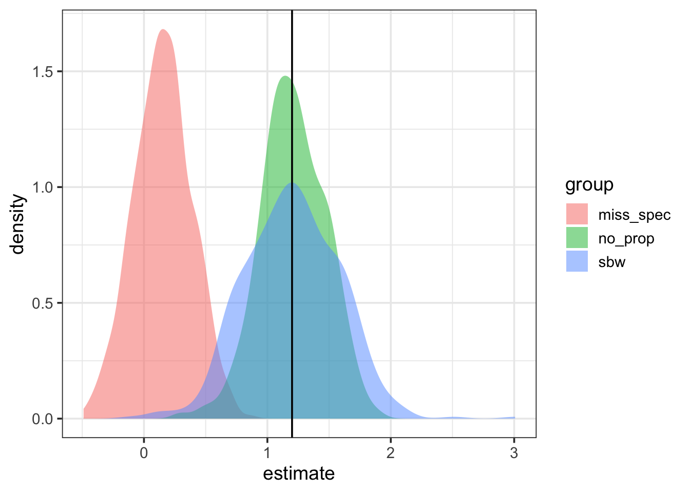
These examples show how simglm can be used not only to simulate propensity score models but also to estimate power under different adjustment strategies. By simulating under known conditions, you can evaluate the robustness of your causal modeling choices before applying them to real data. Because these same simulations can also track significance rates across replications, you can easily extend them to estimate statistical power under different adjustment strategies.
Code
sessionInfo()R version 4.5.0 (2025-04-11)
Platform: aarch64-apple-darwin20
Running under: macOS 26.0.1
Matrix products: default
BLAS: /Library/Frameworks/R.framework/Versions/4.5-arm64/Resources/lib/libRblas.0.dylib
LAPACK: /Library/Frameworks/R.framework/Versions/4.5-arm64/Resources/lib/libRlapack.dylib; LAPACK version 3.12.1
locale:
[1] C.UTF-8/C.UTF-8/C.UTF-8/C/C.UTF-8/C.UTF-8
time zone: America/Chicago
tzcode source: internal
attached base packages:
[1] stats graphics grDevices utils datasets methods base
other attached packages:
[1] future_1.58.0 simglm_0.9.26 ggplot2_4.0.0
loaded via a namespace (and not attached):
[1] utf8_1.2.6 tidyr_1.3.1 generics_0.1.4
[4] gtools_3.9.5 stringi_1.8.7 lattice_0.22-6
[7] hms_1.1.3 listenv_0.9.1 lme4_1.1-37
[10] digest_0.6.37 magrittr_2.0.3 evaluate_1.0.5
[13] grid_4.5.0 RColorBrewer_1.1-3 fastmap_1.2.0
[16] ggformula_0.12.0 jsonlite_2.0.0 Matrix_1.7-3
[19] backports_1.5.0 purrr_1.1.0 scales_1.4.0
[22] codetools_0.2-20 labelled_2.14.1 reformulas_0.4.1
[25] Rdpack_2.6.4 cli_3.6.5 rlang_1.1.6
[28] rbibutils_2.3 parallelly_1.45.0 future.apply_1.20.0
[31] splines_4.5.0 withr_3.0.2 yaml_2.3.10
[34] tools_4.5.0 parallel_4.5.0 nloptr_2.2.1
[37] minqa_1.2.8 dplyr_1.1.4 mosaicCore_0.9.4.0
[40] forcats_1.0.0 boot_1.3-31 globals_0.18.0
[43] broom_1.0.8 vctrs_0.6.5 R6_2.6.1
[46] ggridges_0.5.6 lifecycle_1.0.4 stringr_1.5.2
[49] htmlwidgets_1.6.4 MASS_7.3-65 pkgconfig_2.0.3
[52] pillar_1.11.0 gtable_0.3.6 glue_1.8.0
[55] Rcpp_1.1.0 haven_2.5.4 xfun_0.53
[58] tibble_3.3.0 tidyselect_1.2.1 knitr_1.50
[61] farver_2.1.2 htmltools_0.5.8.1 nlme_3.1-168
[64] labeling_0.4.3 rmarkdown_2.29 compiler_4.5.0
[67] S7_0.2.0