Code
remotes::install_github('lebebr01/simglm')This update marks the final propensity score enhancement for the simglm package (v0.9.26). It introduces multi-level propensity score modeling, enabling users to simulate data with nested structures and treatment effects that vary across levels.
Propensity score methods often assume independence between units, but in real-world settings, data are hierarchical (e.g., students nested in classrooms, patients nested in hospitals). This release bridges that gap—allowing for realistic multi-level causal inference simulation.
propensity_model argument now supports random effects and hierarchical assignment.glm, lme4::glmer, or even brms::brm) with additional arguments.If you haven’t already, remember to first install the latest release of the simglm package from GitHub.
remotes::install_github('lebebr01/simglm')First, let’s show the new features that allow the user to specify a multi-level propensity score model. In this example, we will simulate data with students nested within classrooms, where the treatment assignment is still being specified at the student level. The model formula specified for both the full data generation and propensity model specification use lme4 style syntax. Any data features generated during the propensity score model simulation carry over to the final data generation step.
library(simglm)

level1_samp <- sample(15:25, size = 50, replace = TRUE)

sim_arguments <- list(
    formula = achievement ~ 1 + motivation + trt + age + ses + (1 | classroom),
    fixed = list(
        motivation = list(var_type = 'continuous',
                           mean = 0, sd = 20)
    ),
    sample_size = list(level1 = level1_samp, level2 = 50),
    error = list(variance = 10),
    reg_weights = c(50, 0.4, 1.2, 0.1, 0.25),
    randomeffect = list(int_classroom = list(variance = 5, var_level = 2)),
    propensity = list(
        formula = trt ~ 1 + age + ses + (1 | classroom),
        fixed = list(age = list(var_type = 'ordinal',
                         levels = -7:7),
                     ses = list(var_type = 'continuous',
                         mean = 0, sd = 5,
                         var_level = 2)),
        sample_size = list(level1 = level1_samp, level2 = 50),
        error = list(variance = 5),
        randomeffect = list(int_classroom = list(variance = 5, var_level = 2)),
        reg_weights = c(2, 0.3, -0.5),
        outcome_type = 'binary'
    )
)
simulate_fixed(data = NULL, sim_args = sim_arguments) |>
    simulate_error(sim_args = sim_arguments) |>
    simulate_randomeffect(sim_args = sim_arguments) |>
    generate_response(sim_arguments) |>
    head()
X.Intercept. motivation trt age ses level1_id classroom error
1 1 6.502731 1 -4 1.026945 1 1 -0.9554712
2 1 4.548620 1 2 1.026945 2 1 -5.7521228
3 1 11.132905 0 -2 1.026945 3 1 3.8836490
4 1 -3.523738 0 2 1.026945 4 1 1.6403897
5 1 41.977955 0 -3 1.026945 5 1 -2.5984848
6 1 -8.826909 0 -6 1.026945 6 1 -0.0853880
int_classroom fixed_outcome random_effects achievement
1 -1.405126 53.65783 -1.405126 51.29723
2 -1.405126 53.47618 -1.405126 46.31894
3 -1.405126 54.50990 -1.405126 56.98842
4 -1.405126 49.04724 -1.405126 49.28251
5 -1.405126 66.74792 -1.405126 62.74431
6 -1.405126 46.12597 -1.405126 44.63546In addition to specifying treatment at level 1 (e.g., students), users can now specify treatment assignment at higher levels (e.g., classrooms). Below is an example where treatment is assigned at level 2 (classrooms). The simglm package does this by computing the average value for each cluster (classrooms here) and then uses that value to assign the treatment to that cluster. To specify this treatment assignment, the user simply needs to set the outcome_level argument within the propensity list to the desired level (2 in this case).
level1_samp <- sample(15:25, size = 50, replace = TRUE)

sim_arguments <- list(
    formula = achievement ~ 1 + motivation + trt + age + ses + (1 | classroom),
    fixed = list(
        motivation = list(var_type = 'continuous',
                           mean = 0, sd = 20)
    ),
    sample_size = list(level1 = level1_samp, level2 = 50),
    error = list(variance = 10),
    reg_weights = c(50, 0.4, 1.2, 0.1, 0.25),
    randomeffect = list(int_classroom = list(variance = 5, var_level = 2)),
    propensity = list(
        formula = trt ~ 1 + age + ses + (1 | classroom),
        fixed = list(age = list(var_type = 'ordinal',
                         levels = -7:7),
                     ses = list(var_type = 'continuous',
                         mean = 0, sd = 5,
                         var_level = 2)),
        sample_size = list(level1 = level1_samp, level2 = 50),
        error = list(variance = 5),
        randomeffect = list(int_classroom = list(variance = 5, var_level = 2)),
        reg_weights = c(2, 0.3, -0.5),
        outcome_type = 'binary',
        outcome_level = 2
    )
)
simulate_fixed(data = NULL, sim_args = sim_arguments) |>
    simulate_error(sim_args = sim_arguments) |>
    simulate_randomeffect(sim_args = sim_arguments) |>
    generate_response(sim_arguments)|>
    head()
X.Intercept. motivation trt age ses level1_id classroom error
1 1 23.948833 1 2 -1.499993 1 1 -3.4630538
2 1 3.517415 1 5 -1.499993 2 1 1.0019384
3 1 -12.423001 1 4 -1.499993 3 1 0.4293656
4 1 -23.844401 1 -6 -1.499993 4 1 -0.9232922
5 1 -44.794205 1 3 -1.499993 5 1 1.9578812
6 1 14.122256 1 -5 -1.499993 6 1 -2.1116858
int_classroom fixed_outcome random_effects achievement
1 5.951099 60.60453 5.951099 63.09258
2 5.951099 52.73197 5.951099 59.68500
3 5.951099 46.25580 5.951099 52.63627
4 5.951099 40.68724 5.951099 45.71505
5 5.951099 33.20732 5.951099 41.11630
6 5.951099 55.97390 5.951099 59.81332💡 Tip: When treatment is assigned at a higher level, all units within that cluster receive the same treatment indicator. This makes simulation results especially useful for cluster-randomized trial designs.
Here’s a quick example of how you might visualize simulated treatment variation across classrooms:
sim_data <- simulate_fixed(data = NULL, sim_args = sim_arguments) |>
  simulate_error(sim_args = sim_arguments) |>
  simulate_randomeffect(sim_args = sim_arguments) |>
  generate_response(sim_arguments)

ggplot(sim_data, aes(x = factor(classroom), y = trt)) +
  geom_boxplot() +
  labs(
    x = "Classroom ID",
    y = "Treatment Assignment (0 = Control, 1 = Treatment)",
    title = "Cluster-Level Treatment Variation"
  )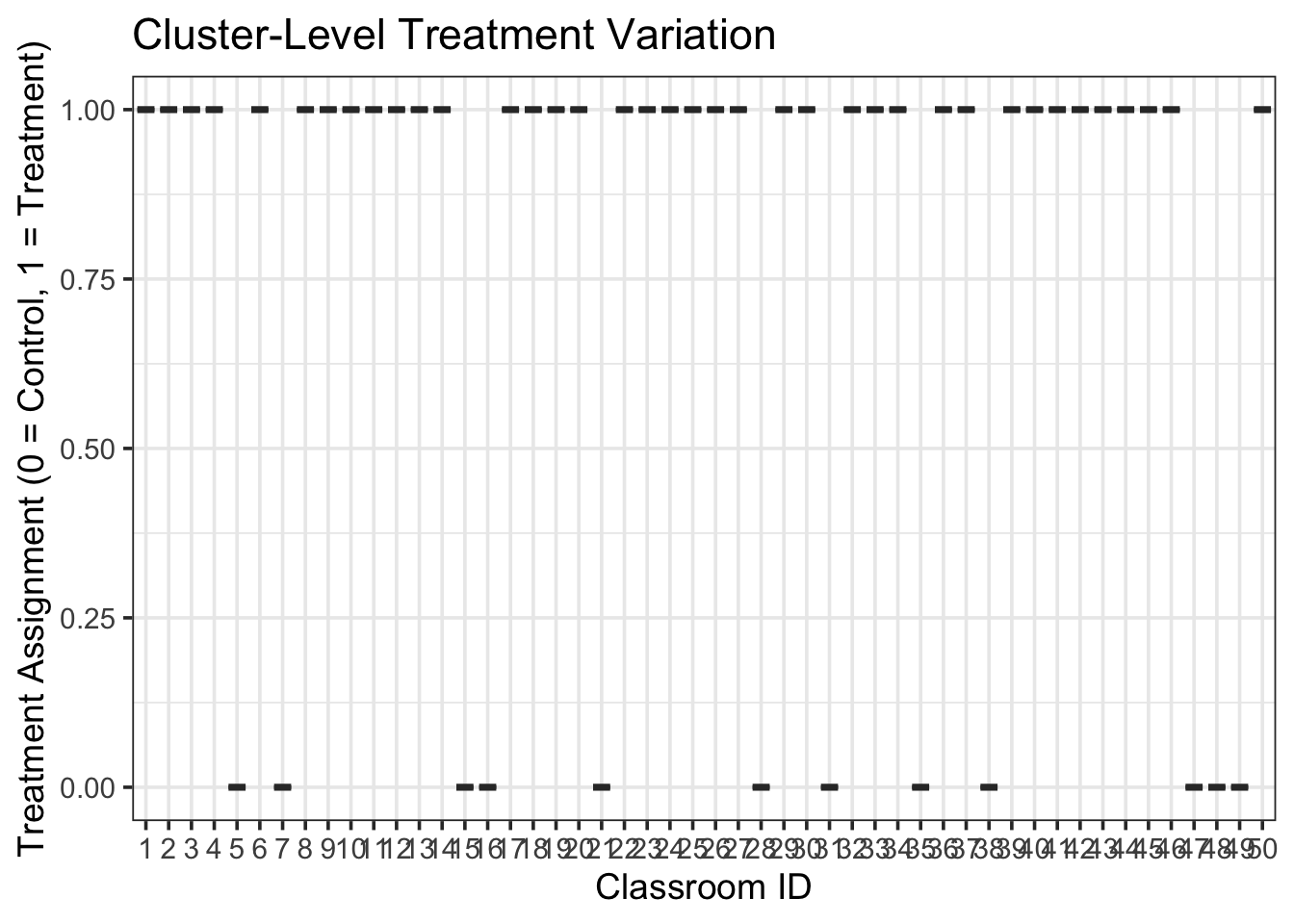
Here is an example where there are now classrooms and districts being specified. The treatment assignment is still being specified at the classroom level with outcome_level = 2, but there is now another level to be considered.
level1_samp <- sample(15:25, size = 150, replace = TRUE)

sim_arguments <- list(
    formula = achievement ~ 1 + motivation + trt + age + ses + (1 | classroom) + (1 | district),
    fixed = list(
        motivation = list(var_type = 'continuous',
                           mean = 0, sd = 20)
    ),
    sample_size = list(level1 = level1_samp, level2 = 10, level3 = 15),
    error = list(variance = 10),
    reg_weights = c(50, 0.4, 1.2, 0.1, 0.25),
    randomeffect = list(int_classroom = list(variance = 5, var_level = 2),
    int_district = list(variance = 2, var_level = 3)),
    propensity = list(
        formula = trt ~ 1 + age + ses + (1 | classroom) + (1 | district),
        fixed = list(age = list(var_type = 'ordinal',
                         levels = -7:7),
                     ses = list(var_type = 'continuous',
                         mean = 0, sd = 5,
                         var_level = 2)),
        sample_size =  list(level1 = level1_samp, level2 = 10, level3 = 15),
        error = list(variance = 5),
        randomeffect = list(int_classroom = list(variance = 5, var_level = 2),
        int_district = list(variance = 2, var_level = 3)),
        reg_weights = c(2, 0.3, -0.5),
        outcome_type = 'binary',
        outcome_level = 2
    )
)
simulate_fixed(data = NULL, sim_args = sim_arguments) |>
    simulate_error(sim_args = sim_arguments) |>
    simulate_randomeffect(sim_args = sim_arguments) |>
    generate_response(sim_arguments) |>
    head()
New names:
New names:
• `X.Intercept.` -> `X.Intercept....1`
• `X.Intercept.` -> `X.Intercept....2` X.Intercept. motivation trt age ses level1_id classroom district
1 1 -54.488721 1 -1 -5.700812 1 1 1
2 1 -5.005362 1 -1 -5.700812 2 1 1
3 1 37.278043 1 -2 -5.700812 3 1 1
4 1 -20.904998 1 5 -5.700812 4 1 1
5 1 12.779405 1 -7 -5.700812 5 1 1
6 1 4.861477 1 -7 -5.700812 6 1 1
error int_classroom int_district fixed_outcome random_effects achievement
1 -7.056390 1.836647 0.2612293 27.87931 2.097876 22.92079
2 -4.276418 1.836647 0.2612293 47.67265 2.097876 45.49411
3 4.207792 1.836647 0.2612293 64.48601 2.097876 70.79168
4 3.465661 1.836647 0.2612293 41.91280 2.097876 47.47634
5 2.112933 1.836647 0.2612293 54.18656 2.097876 58.39737
6 -1.283107 1.836647 0.2612293 51.01939 2.097876 51.83416The treatment assignment can alternatively be specified at the district level, by setting outcome_level = 3 within the propensity list.
level1_samp <- sample(15:25, size = 150, replace = TRUE)

sim_arguments <- list(
    formula = achievement ~ 1 + motivation + trt + age + ses + (1 | classroom) + (1 | district),
    fixed = list(
        motivation = list(var_type = 'continuous',
                           mean = 0, sd = 20)
    ),
    sample_size = list(level1 = level1_samp, level2 = 10, level3 = 15),
    error = list(variance = 10),
    reg_weights = c(50, 0.4, 1.2, 0.1, 0.25),
    randomeffect = list(int_classroom = list(variance = 5, var_level = 2),
    int_district = list(variance = 2, var_level = 3)),
    propensity = list(
        formula = trt ~ 1 + age + ses + (1 | classroom) + (1 | district),
        fixed = list(age = list(var_type = 'ordinal',
                         levels = -7:7),
                     ses = list(var_type = 'continuous',
                         mean = 0, sd = 5,
                         var_level = 2)),
        sample_size =  list(level1 = level1_samp, level2 = 10, level3 = 15),
        error = list(variance = 5),
        randomeffect = list(int_classroom = list(variance = 5, var_level = 2),
        int_district = list(variance = 2, var_level = 3)),
        reg_weights = c(2, 0.3, -0.5),
        outcome_type = 'binary',
        outcome_level = 3
    )
)
simulate_fixed(data = NULL, sim_args = sim_arguments) |>
    simulate_error(sim_args = sim_arguments) |>
    simulate_randomeffect(sim_args = sim_arguments) |>
    generate_response(sim_arguments)|>
    head()
New names:
New names:
• `X.Intercept.` -> `X.Intercept....1`
• `X.Intercept.` -> `X.Intercept....2` X.Intercept. motivation trt age ses level1_id classroom district
1 1 -4.538476 1 7 1.670979 1 1 1
2 1 -9.869254 1 3 1.670979 2 1 1
3 1 -6.006584 1 3 1.670979 3 1 1
4 1 16.765529 1 2 1.670979 4 1 1
5 1 -9.933779 1 -3 1.670979 5 1 1
6 1 34.817235 1 5 1.670979 6 1 1
error int_classroom int_district fixed_outcome random_effects
1 1.7127887 4.874151 -0.98758 50.50235 3.886571
2 -2.5383693 4.874151 -0.98758 47.97004 3.886571
3 0.3557401 4.874151 -0.98758 49.51511 3.886571
4 -3.2642383 4.874151 -0.98758 58.52396 3.886571
5 1.2402380 4.874151 -0.98758 47.34423 3.886571
6 -5.6804034 4.874151 -0.98758 66.04464 3.886571
achievement
1 56.10171
2 49.31824
3 53.75742
4 59.14629
5 52.47104
6 64.25081The other enhancement is to how the propensity model is fitted and extracted. The internal function for this process has been generalized to allow users to specify whichever model fitting procedure they want. If no model fitting is specified, stats::glm() function is used. If there is a multi-level structure, lme4::glmer() or some alternative, would be more appropriate and would need to be specified within the propensity_model simulation arguments.
level1_samp <- sample(15:25, size = 75, replace = TRUE)

sim_arguments <- list(
    formula = achievement ~ 1 + motivation + trt + age + ses + (1 | classroom),
    fixed = list(
        motivation = list(var_type = 'continuous',
                           mean = 0, sd = 20)
    ),
    sample_size = list(level1 = level1_samp, level2 = 75),
    error = list(variance = 10),
    reg_weights = c(0, 0.4, 1.2, 0.1, 0.25),
    randomeffect = list(int_classroom = list(variance = 5, var_level = 2)),
    propensity = list(
        formula = trt ~ 1 + age + ses + (1 | classroom),
        fixed = list(age = list(var_type = 'ordinal',
                         levels = -7:7),
                     ses = list(var_type = 'continuous',
                         mean = 0, sd = 5,
                         var_level = 2)),
        sample_size = list(level1 = level1_samp, level2 = 75),
        error = list(variance = 10),
        randomeffect = list(int_classroom = list(variance = 5, var_level = 2)),
        reg_weights = c(2, 0.5, -0.8),
        outcome_type = 'binary',
        outcome_level = 2
    ),
    model_fit = list(formula = achievement ~ 1 + motivation + trt + (1 | classroom),
                   model_function = lme4::lmer),
    propensity_model = list(
        formula = trt ~ 1 + age + ses + (1 | classroom),
        propensity_type = 'covariate',
        model_function = lme4::glmer,
        propensity_model_args = list(
           family = binomial()
        )
    ),
    replications = 10,
    extract_coefficients = TRUE
)

replicate_simulation(sim_arguments)
Warning in checkConv(attr(opt, "derivs"), opt$par, ctrl = control$checkConv, :
Model failed to converge with max|grad| = 0.0556873 (tol = 0.002, component 1)Warning in checkConv(attr(opt, "derivs"), opt$par, ctrl = control$checkConv, : Model is nearly unidentifiable: very large eigenvalue
- Rescale variables?[[1]]
term estimate std.error statistic
1 (Intercept) 2.908904e+00 7.138991e-01 4.074670
2 motivation 4.056633e-01 4.302511e-03 94.285228
3 trt 2.369709e+04 6.787640e+03 3.491212
4 propensity -2.369950e+04 6.788101e+03 -3.491329
[[2]]
term estimate std.error statistic
1 (Intercept) 1.256255e+00 4.501801e-01 2.790561
2 motivation 3.988186e-01 4.456008e-03 89.501326
3 trt 1.035445e+04 6.851057e+03 1.511366
4 propensity -1.035536e+04 6.851238e+03 -1.511458
[[3]]
term estimate std.error statistic
1 (Intercept) 9.734051e-01 5.325444e-01 1.827838
2 motivation 4.034641e-01 4.247209e-03 94.995117
3 trt 1.522479e+04 9.038478e+03 1.684441
4 propensity -1.522510e+04 9.038724e+03 -1.684430
[[4]]
term estimate std.error statistic
1 (Intercept) 1.2694900 4.291298e-01 2.958289
2 motivation 0.3971322 4.178960e-03 95.031348
3 trt 5118.1511922 3.557972e+03 1.438502
4 propensity -5118.8380437 3.558231e+03 -1.438591
[[5]]
term estimate std.error statistic
1 (Intercept) 1.4644805 5.567131e-01 2.6305841
2 motivation 0.3982062 4.077144e-03 97.6679352
3 trt 2105.2649994 7.100847e+03 0.2964808
4 propensity -2106.0079375 7.101062e+03 -0.2965765
[[6]]
term estimate std.error statistic
1 (Intercept) 0.8776863 5.054796e-01 1.736343
2 motivation 0.3955913 4.261973e-03 92.818811
3 trt 3796.5598590 2.271809e+03 1.671162
4 propensity -3797.5932828 2.272149e+03 -1.671367
[[7]]
term estimate std.error statistic
1 (Intercept) 1.1598000 4.936926e-01 2.349235
2 motivation 0.4055483 4.287862e-03 94.580542
3 trt 6389.5839804 2.894362e+03 2.207597
4 propensity -6390.3572335 2.894661e+03 -2.207636
[[8]]
term estimate std.error statistic
1 (Intercept) 2.024031e+00 4.310026e-01 4.696100
2 motivation 4.006582e-01 4.150963e-03 96.521753
3 trt 1.704448e+04 6.978264e+03 2.442510
4 propensity -1.704617e+04 6.978520e+03 -2.442663
[[9]]
term estimate std.error statistic
1 (Intercept) 1.001839e+00 5.212012e-01 1.922172
2 motivation 4.024457e-01 4.201464e-03 95.786999
3 trt 1.776691e+04 8.062954e+03 2.203524
4 propensity -1.776733e+04 8.063197e+03 -2.203509
[[10]]
term estimate std.error statistic
1 (Intercept) 2.475772e+00 6.106023e-01 4.054639
2 motivation 4.004046e-01 4.167494e-03 96.078010
3 trt 1.989337e+04 7.453907e+03 2.668851
4 propensity -1.989594e+04 7.454200e+03 -2.669091brmsIt is also possible to use different model fitting functions. For example, if you wanted to use a Bayesian logistic regression function, this is now possible with the new model fitting functionality. I’m going to use the example from the last post with single level propensity score models to demonstrate this feature. Here, I will use the brms::brm() function to fit a Bayesian logistic regression model for the propensity score model.
sim_arguments <- list(
    formula = achievement ~ 1 + motivation + trt + age + ses,
    fixed = list(
        motivation = list(var_type = 'continuous',
                           mean = 0, sd = 20)
    ),
    sample_size = 400,
    error = list(variance = 10),
    reg_weights = c(50, 0.4, 1.2, 0.1, 0.25),
    propensity = list(
        formula = trt ~ 1 + age + ses,
        fixed = list(age = list(var_type = 'ordinal',
                         levels = -7:7),
                     ses = list(var_type = 'continuous',
                         mean = 0, sd = 5)),
        sample_size = 400,
        error = list(variance = 5),
        reg_weights = c(2, 0.3, -0.5),
        outcome_type = 'binary'
    ),
    model_fit = list(formula = achievement ~ 1 + motivation + trt + age + ses,
                   model_function = 'lm'),
    propensity_model = list(
        formula = trt ~ 1 + age + ses,
        propensity_type = 'sbw',
        model_function = brms::brm,
    propensity_model_args = list(iter = 250, chains = 2, family = brms::bernoulli())
    ),
    replications = 2,
    extract_coefficients = TRUE
)
replicate_simulation(sim_arguments)
SAMPLING FOR MODEL 'anon_model' NOW (CHAIN 1).
Chain 1:
Chain 1: Gradient evaluation took 2.2e-05 seconds
Chain 1: 1000 transitions using 10 leapfrog steps per transition would take 0.22 seconds.
Chain 1: Adjust your expectations accordingly!
Chain 1:
Chain 1:
Chain 1: WARNING: There aren't enough warmup iterations to fit the
Chain 1:          three stages of adaptation as currently configured.
Chain 1:          Reducing each adaptation stage to 15%/75%/10% of
Chain 1:          the given number of warmup iterations:
Chain 1:            init_buffer = 18
Chain 1:            adapt_window = 95
Chain 1:            term_buffer = 12
Chain 1:
Chain 1: Iteration:   1 / 250 [  0%]  (Warmup)
Chain 1: Iteration:  25 / 250 [ 10%]  (Warmup)
Chain 1: Iteration:  50 / 250 [ 20%]  (Warmup)
Chain 1: Iteration:  75 / 250 [ 30%]  (Warmup)
Chain 1: Iteration: 100 / 250 [ 40%]  (Warmup)
Chain 1: Iteration: 125 / 250 [ 50%]  (Warmup)
Chain 1: Iteration: 126 / 250 [ 50%]  (Sampling)
Chain 1: Iteration: 150 / 250 [ 60%]  (Sampling)
Chain 1: Iteration: 175 / 250 [ 70%]  (Sampling)
Chain 1: Iteration: 200 / 250 [ 80%]  (Sampling)
Chain 1: Iteration: 225 / 250 [ 90%]  (Sampling)
Chain 1: Iteration: 250 / 250 [100%]  (Sampling)
Chain 1:
Chain 1:  Elapsed Time: 0.004 seconds (Warm-up)
Chain 1:                0.003 seconds (Sampling)
Chain 1:                0.007 seconds (Total)
Chain 1:

SAMPLING FOR MODEL 'anon_model' NOW (CHAIN 2).
Chain 2:
Chain 2: Gradient evaluation took 6e-06 seconds
Chain 2: 1000 transitions using 10 leapfrog steps per transition would take 0.06 seconds.
Chain 2: Adjust your expectations accordingly!
Chain 2:
Chain 2:
Chain 2: WARNING: There aren't enough warmup iterations to fit the
Chain 2:          three stages of adaptation as currently configured.
Chain 2:          Reducing each adaptation stage to 15%/75%/10% of
Chain 2:          the given number of warmup iterations:
Chain 2:            init_buffer = 18
Chain 2:            adapt_window = 95
Chain 2:            term_buffer = 12
Chain 2:
Chain 2: Iteration:   1 / 250 [  0%]  (Warmup)
Chain 2: Iteration:  25 / 250 [ 10%]  (Warmup)
Chain 2: Iteration:  50 / 250 [ 20%]  (Warmup)
Chain 2: Iteration:  75 / 250 [ 30%]  (Warmup)
Chain 2: Iteration: 100 / 250 [ 40%]  (Warmup)
Chain 2: Iteration: 125 / 250 [ 50%]  (Warmup)
Chain 2: Iteration: 126 / 250 [ 50%]  (Sampling)
Chain 2: Iteration: 150 / 250 [ 60%]  (Sampling)
Chain 2: Iteration: 175 / 250 [ 70%]  (Sampling)
Chain 2: Iteration: 200 / 250 [ 80%]  (Sampling)
Chain 2: Iteration: 225 / 250 [ 90%]  (Sampling)
Chain 2: Iteration: 250 / 250 [100%]  (Sampling)
Chain 2:
Chain 2:  Elapsed Time: 0.004 seconds (Warm-up)
Chain 2:                0.003 seconds (Sampling)
Chain 2:                0.007 seconds (Total)
Chain 2:

SAMPLING FOR MODEL 'anon_model' NOW (CHAIN 1).
Chain 1:
Chain 1: Gradient evaluation took 1.8e-05 seconds
Chain 1: 1000 transitions using 10 leapfrog steps per transition would take 0.18 seconds.
Chain 1: Adjust your expectations accordingly!
Chain 1:
Chain 1:
Chain 1: WARNING: There aren't enough warmup iterations to fit the
Chain 1:          three stages of adaptation as currently configured.
Chain 1:          Reducing each adaptation stage to 15%/75%/10% of
Chain 1:          the given number of warmup iterations:
Chain 1:            init_buffer = 18
Chain 1:            adapt_window = 95
Chain 1:            term_buffer = 12
Chain 1:
Chain 1: Iteration:   1 / 250 [  0%]  (Warmup)
Chain 1: Iteration:  25 / 250 [ 10%]  (Warmup)
Chain 1: Iteration:  50 / 250 [ 20%]  (Warmup)
Chain 1: Iteration:  75 / 250 [ 30%]  (Warmup)
Chain 1: Iteration: 100 / 250 [ 40%]  (Warmup)
Chain 1: Iteration: 125 / 250 [ 50%]  (Warmup)
Chain 1: Iteration: 126 / 250 [ 50%]  (Sampling)
Chain 1: Iteration: 150 / 250 [ 60%]  (Sampling)
Chain 1: Iteration: 175 / 250 [ 70%]  (Sampling)
Chain 1: Iteration: 200 / 250 [ 80%]  (Sampling)
Chain 1: Iteration: 225 / 250 [ 90%]  (Sampling)
Chain 1: Iteration: 250 / 250 [100%]  (Sampling)
Chain 1:
Chain 1:  Elapsed Time: 0.004 seconds (Warm-up)
Chain 1:                0.003 seconds (Sampling)
Chain 1:                0.007 seconds (Total)
Chain 1:

SAMPLING FOR MODEL 'anon_model' NOW (CHAIN 2).
Chain 2:
Chain 2: Gradient evaluation took 5e-06 seconds
Chain 2: 1000 transitions using 10 leapfrog steps per transition would take 0.05 seconds.
Chain 2: Adjust your expectations accordingly!
Chain 2:
Chain 2:
Chain 2: WARNING: There aren't enough warmup iterations to fit the
Chain 2:          three stages of adaptation as currently configured.
Chain 2:          Reducing each adaptation stage to 15%/75%/10% of
Chain 2:          the given number of warmup iterations:
Chain 2:            init_buffer = 18
Chain 2:            adapt_window = 95
Chain 2:            term_buffer = 12
Chain 2:
Chain 2: Iteration:   1 / 250 [  0%]  (Warmup)
Chain 2: Iteration:  25 / 250 [ 10%]  (Warmup)
Chain 2: Iteration:  50 / 250 [ 20%]  (Warmup)
Chain 2: Iteration:  75 / 250 [ 30%]  (Warmup)
Chain 2: Iteration: 100 / 250 [ 40%]  (Warmup)
Chain 2: Iteration: 125 / 250 [ 50%]  (Warmup)
Chain 2: Iteration: 126 / 250 [ 50%]  (Sampling)
Chain 2: Iteration: 150 / 250 [ 60%]  (Sampling)
Chain 2: Iteration: 175 / 250 [ 70%]  (Sampling)
Chain 2: Iteration: 200 / 250 [ 80%]  (Sampling)
Chain 2: Iteration: 225 / 250 [ 90%]  (Sampling)
Chain 2: Iteration: 250 / 250 [100%]  (Sampling)
Chain 2:
Chain 2:  Elapsed Time: 0.004 seconds (Warm-up)
Chain 2:                0.004 seconds (Sampling)
Chain 2:                0.008 seconds (Total)
Chain 2:
[[1]]
# A tibble: 5 × 5
term estimate std.error statistic p.value
<chr> <dbl> <dbl> <dbl> <dbl>
1 (Intercept) 50.4 0.405 124. 5.47e-319
2 motivation 0.410 0.00830 49.4 3.16e-171
3 trt 0.542 0.514 1.05 2.92e- 1
4 age 0.152 0.0456 3.33 9.58e- 4
5 ses 0.194 0.0350 5.54 5.39e- 8
[[2]]
# A tibble: 5 × 5
term estimate std.error statistic p.value
<chr> <dbl> <dbl> <dbl> <dbl>
1 (Intercept) 50.6 0.379 133. 0
2 motivation 0.405 0.00855 47.3 7.05e-165
3 trt 0.288 0.474 0.606 5.45e- 1
4 age 0.109 0.0435 2.52 1.23e- 2
5 ses 0.159 0.0402 3.96 9.02e- 5⚙️ Note: For demonstration purposes, this example uses only 2 replications and 250 iterations across 2 chains. For accurate estimation, these should be increased substantially.
These enhancements make simglm a more powerful framework for propensity score simulation, causal inference, and power analysis in multi-level contexts. You can now simulate, estimate, and evaluate designs involving cluster-level assignment, cross-level effects, and complex hierarchical data structures—all within a single pipeline!